Activity identification using body
mounted sensors — a review of
classification techniques
Preece, SJ, Goulermas, JY, Kenney, LPJ, Howard, D, Meijer, K and Crompton, R
http://dx.doi.org/10.1088/09673334/30/4/R01
Title
Activity identification using bodymounted sensors — a review of
classification techniques
Authors
Preece, SJ, Goulermas, JY, Kenney, LPJ, Howard, D, Meijer, K and
Crompton, R
Type
Article
URL
This version is available at: http://usir.salford.ac.uk/12572/
Published Date
2009
USIR is a digital collection of the research output of the University of Salford. Where copyright
permits, full text material held in the repository is made freely available online and can be read,
downloaded and copied for noncommercial private study or research purposes. Please check the
manuscript for any further copyright restrictions.
Title:
Activity identification using body-mounted sensors – a review of classification techniques
Article Type:
Topical Review
Keywords:
Activity monitoring, classification, falls detection, machine learning
Abstract
Table of contents
1. Introduction 2. Body-worn sensors
2.1 Inertial sensors 2.2 Other sensors 3. Windowing Techniques 4. Feature Generation
4.1 Heuristic features 4.2 Time-domain features 4.3 Frequency-domain features
4.4 Wavelet analysis (Time-frequency features) 4.5 Feature selection methods
4.6 Dimensionality reduction methods 5. Classification Schemes
5.1 Threshold-based classification 5.2 Hierarchical methods
5.3 Decision trees 5.4 k-Nearest Neighbour 5.5 Artificial neural networks 5.6 Support Vector Machines
5.7 Naive Bayes and Gaussian mixture models 5.8 Fuzzy Logic
5.9 Markov Chains and Hidden Markov Models 5.10 Combining Different Classifiers
5.11 Unsupervised learning
Activity identification using body-mounted sensors – a review of classification
techniques
1. Introduction
Physical activity has been defined as “any bodily movement produced by skeletal muscles that results in energy expenditure above resting level” (Caspersen et al 1985). Activity classification is a recent concept involving the use of technology to automatically recognise different activities and, in some cases, to collate this information into a continuous record. The need for automated activity classification systems has been identified in a number of different fields, from health-related research to pervasive computing, as discussed below.
With the shift towards more sedentary lifestyles in both developed and developing nations, there is a need for research investigating the links between common diseases and levels of physical activity. Conditions such as cardiovascular disease (Barengo et al 2004), hypertension (Blair et al 1984), diabetes mellitus (Manson et al
1991) and depression (Yancey et al 2004) have all been linked to physical inactivity. Although some epidemiological studies have used self reporting (diaries) to quantify activity patterns, these methods have been shown to be unreliable (Ainsworth et al 1993; Washburn and Montoye 1986). Instead, fully automated activity classification offers a more objective approach to quantifying levels of physical activity.
Activity classification systems can also be used to investigate the effectiveness of initiatives aimed at increasing physical activity (van Sluijs et al 2007). A better understanding of why people choose to exercise and how individuals can be motivated to increase their levels of physical activity is crucial if the current health epidemic resulting from physical inactivity is to be reversed (Dugdill et al 2009). Furthermore, activity classification systems could be used to provide feedback to motivate individuals to adhere to daily or weekly physical activity targets (Baker and Mutrie 2005).
systems have been used in patients with Parkinson’s disease (Dunnewold et al 1997; Moore et al 2008) and to validate the use of different motor subtypes in delirium (Leonard et al 2007). They have also been shown to be a valid in the assessment of physical activity levels in patients with multiple sclerosis (Ng and Kent-Braun 1997), osteoarthritis (Brandes et al 2008) and chronic pulmonary disease (Pitta et al 2006). Furthermore, automated activity classification systems have considerable potential to be used to assess effectiveness of treatments. For example, in stroke, accelerometer-based systems can be used to recognise real-world upper extremity movement which could then be used to derive treatment outcomes (Uswatte et al
2000).
With an aging population the incidence of falls is increasing. As many elderly persons now live alone, falls can go undetected and injured individuals left unaided for lengthy periods of time (Gurley et al 1996). Research has shown that the earlier a fall is reported the lower the rate of morbidity and mortality (Gurley et al 1996; Wild et al 1981). Clearly, any system which can accurately detect a fall and automatically call for help could be of major benefit. A fall is not an intentional movement; however, within the context of activity classification, it can be considered a specific form of activity. As such, the analytical techniques used in activity classification are also applicable to fall detection systems.
In addition to health-related applications, activity profiling systems could play a fundamental role in ubiquitous computing scenarios (Coutaz et al 2005; Streitz and Nixon 2005). In such applications information from a variety of sensors is used to determine the context of a situation, so that an appropriate service can be provided. For example, a mobile phone may detect when a person is driving or involved in vigorous physical activity and automatically divert a call.
data can be used for estimating functional parameters, such as gait speed and energy expenditure, and for activity classification to produce a continuous activity record. The focus of this review is activity classification. Other methods for interpreting body-worn sensor data are reviewed elsewhere, for example Chen and Bassett (2005) and Kavanagh and Menz (2008).
The automated identification of activities using body-worn sensor data is a challenging area of work. Apart from the obvious practical limitations on the number, location and nature of sensors that people will tolerate there are several issues that directly impact of the success of any given algorithm. Problems arise due to the variability in sensor characteristics for the same activity across different subjects and for the same individual. Errors can also arise due to variability in sensor signals caused by differences in sensor positioning and from environmental factors such as sensor temperature sensitivity. Any successful algorithm must overcome all these factors. The ideal activity classification scheme works off-the-shelf, using data from a range of previous subjects to identify activities from an unseen individual. However, sometimes this is not possible and an intra-subject classification scheme is currently all that can be achieved for some problems. With this approach, example data is required for a given individual before classification can be performed.
The aim of this review is to present a conceptual introduction to the different computational techniques that have been applied to activity classification. For this reason, the paper is organised by analytical technique rather than by classification problem. The wide variation in choice of activities between previously published studies means it is not possible to identify a single, optimal solution for any given classification problem. Nevertheless, where appropriate we have tried to provide the reader with a degree of guidance as to the advantages of each of the classification techniques.
we present different approaches to generating features from sensor data and, in Section 5, the classification techniques are described.
2. Body-Worn Sensors
2.1 Inertial sensors
The vast majority of activity classification systems have used inertial sensors, notably accelerometers and rate gyros. Most accelerometers respond to gravity as well as to their true acceleration and, therefore, if the acceleration of the body segment is small with respect to g (9.81m/s2), as is the case when measuring body
sway or static posture, these devices can be used to estimate the inclination of a body segment from the vertical. When the acceleration component becomes large, more sophisticated approaches to separating the orientation component (g) from body segment acceleration are possible. For a detailed description of accelerometry the reader is directed to a comprehensive review by Mathie et al (2004b).
Rate gyro based measurements of angular velocity are subject to significant calibration errors, electronic noise and temperature-effects (Woodman 2007). This means that, if the output is simply integrated to estimate a change in orientation, then the gyro error will be integrated leading to a continuously increasing error. Therefore, integration of rate gyro outputs to estimate orientation changes can only be done over short time periods. A number of approaches have been proposed to overcome this problem including the use of a state estimator with input from a tri-axial gyroscope and a tri-axial accelerometer (Luinge and Veltink 2005) and the use of wavelet analysis (Section 4.4) to remove both drift and high frequency noise from gyroscope signals (Najafi et al 2002) before integrating to obtain orientation.
Inertial sensors can be complemented by a magnetic compass or magnetometer (Parkka et al 2006), which can enable more accurate orientation measurement about the vertical axis (Sabatini 2006) and by GPS (Murakami and Makikawa 1997) to enable location tracking.
Although inertial sensors have been used in the vast majority of activity classification studies, other sensors which may be considered include devices for measuring: segment angles, such as inclinometers (Dai et al
1996) and goniometers (Kostov et al 1995); skin temperature (Krause et al 2003); galvanic skin resistance (Dolgov and Zane 2006), heart rate (Bussmann et al 1998b); humidity (Lester et al 2006); or respiratory rate (Parkka et al 2006).
Recently the concept of ‘smart textiles’ has been proposed, in which miniature sensors are distributed and integrated into clothing (Wijesiriwardana et al 2003). The strict limitation on the size of such integrated sensors means it may not be currently possible to use accelerometers or rate gyroscopes. As an alternative smaller binary sensors, such as tilt switches, have been proposed (van Laerhoven and Cakmakci 2000; van Laerhoven et al 2006).
Simple foot pressure switches can be used to identify gait events such as heel strike and toe off (Mansfield and Lyons 2003). However, as they do not give additional information on limb movement, it is not possible to classify different activities from these signals alone. More detailed information, such as net ground reaction force, can be obtained from pressure sensitive insoles which can assess the pressure distribution across the planter aspect of the foot (Veltink et al 2005; Zhang et al 2005).
3 Windowing Techniques
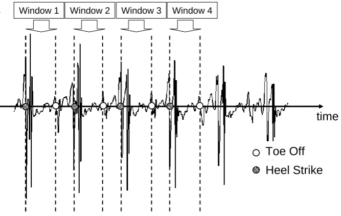
Three different windowing techniques have been used in activity monitoring, sliding windows, event-defined windows and activity-defined windows. With the sliding window method, the signal is divided into windows of fixed length with no inter-window gaps (Figure 1a). A range of window sizes have been used in previous studies from 0.25 secs (Huynh and Schiele 2005) to 6.7 secs (Bao and Intille 2004), with some studies including a degree of overlap between adjacent windows (Bao and Intille 2004; Preece et al 2008b). The sliding widow approach does not require pre-processing of the sensor signal and is therefore ideally suited to real-time applications. Due to its implementational simplicity, most activity classification studies have employed this approach
In order to use event-defined windows, pre-processing is required to locate specific events, such as heel strike or toe-off. These events are then used to define successive windows (Figure 1b). Given that such events may not be uniformly spaced in time, the size of these windows is not fixed. A number of different approaches have been proposed for identifying heel strike and toe off from body-worn sensor signals. For example, it is possible to define search windows from either a low pass filtered version of the original signal (Aminian et al 1999a; Selles et al 2005) or segmental angles (Jasiewicz et al 2006), within which maxima or minima correspond to gait events. Another approach is to identify the times at which the anterio-posterior component of the trunk acceleration changes sign. Heel strike is then located at a given time offset from these points (Mansfield and Lyons 2003; Zijlstra 2004; Zijlstra and Hof 2003).
FIGURE 1 ABOUT HERE
4 Feature Generation
Previous activity classification studies have used a wide range of approaches to generate features which characterise windows of body fixed sensor data. These features are then used as inputs to classification schemes (Section 5). In this section the different feature generation techniques are presented within a number of different sub-categories. Firstly, heuristic features, for both the recognition of everyday activities and falls, are discussed. In this article we use the term heuristic to refer to features which have been derived from a fundamental and often intuitive understanding of how a specific movement or posture will produce a characteristic body-worn sensor signal. In sections 4.2-4.4 domain, frequency-domain and time-frequency (wavelet) features are described. In contrast to the heuristic approach, these features are not typically related to specific aspects of individual movements or postures. Instead they simply represent different ways of characterising the information within the time-varying signal. For a given classification problem it is often difficult to identify optimal time- and frequency-domain features. Therefore methods for selecting optimal features from a larger set and methods for reducing dimensionality of features can be used for pre-processing before advanced classification algorithms are applied. These two techniques are described in section 4.5 and 4.6.
4.1 Heuristic features
Change in segmental orientation can be obtained by integrating a gyroscope signal, provided some method is used to eliminate drift. This feature can then be used to identify different postures and postural transitions (Najafi et al 2002; Najafi et al 2003). As explained earlier, a gyroscope utilises the Coriolois force to quantify segmental angular velocity. Activities which exhibit unique patterns of angular velocity can thus be identified using this feature with a simple classification algorithm, such as a threshold-based classifier. This idea was exploited by Coley et al (2005) who demonstrated that the peak shank angular velocity in the anterior-posterior direction at midstance was positive during stair ascent but negative during level walking and stair descent.
All movement patterns result in time varying segmental accelerations. A number of different methods have been used to derive features which quantify the amplitude of these accelerations. Before these features are derived the signal is first high pass filtered (typically 0.2-0.5Hz) to remove any baseline offset. The range of different features includes signal magnitude area (the area under the high pass filtered acceleration curve) (Mathie et al 2003; Preece et al 2008c), peak-to-peak acceleration (Makikawa and Iizumi 1995), mean rectified value (Bussmann et al 1998a; Bussmann et al 1998b) and root mean square (Veltink et al 1996). This type of feature is often used to differentiate between static and dynamic activity (Mathie et al 2003).
As well as being used as input to classification algorithms, the signal magnitude area (SMA) can be used to quantify the level of intensity of physical activity. This measure is normally expressed in units known as activity counts. It is now well established that, for a given activity, a linear model can be used to relate metabolic energy expenditure to the number of activity counts (Bouten et al 1997; Hendelman et al 2000; Terrier et al 2001). For an excellent review of this area the reader is directed to Chen and Bassett (2005).
The development of robust algorithms which can accurately differentiate between everyday activities and falls using body-worn sensor data is a rapidly growing area of study. The vast majority of previously
ground. In addition there is also a measurable change in the orientation of a number of body segments. Using accelerometers or gyroscopes mounted at the wrist (Degen et al 2003), waist (Karantonis et al 2006), chest (Bourke and Lyons 2008; Bourke et al 2007) or head (Lindemann et al 2005), it is possible to characterise these different events. Typically, a threshold-based classifier (Section 5.1) is then applied to differentiate between falls and everyday activities.
4.2 Time-domain features
Time-domain features are derived directly from a window of sensor data and are typically statistical measures. Example time-domain features used in activity monitoring include the mean, median, variance, skewness, kurtosis (Baek et al 2004; Herren et al 1999) and inter-quartile range (Maurer et al 2006). Other studies have used high and low pass filters to separate accelerometer signals on a frequency basis. Separate means for the low frequency and rectified high frequency components are then used as inputs to the classification schemes (Fahrenberg et al 1997; Foerster and Fahrenberg 2000; Lee et al 2003).
As an alternative to the above, Veltink et al (1996) developed a classification scheme based on measures of signal morphology. With this approach a cross-correlation coefficient was used to quantify the similarity of an event-defined window of data to a previously obtained template signal for each activity. In general, it has been suggested that measures of correlation between different accelerometer axes can improve activity recognition (Aminian et al 1995; Herren et al 1999). Following this idea Bao and Intille (2004) used cross-correlation coefficients to quantify the similarity between acceleration signals from different axes on the same body segment and across different segments.
4.3 Frequency-domain features
distribution from these coefficients. For example, median frequency (Foerster and Fahrenberg 2000) or a subset of the different FFT coefficients can be used (Preece et al 2008a, b) (Preece et al., 2008b, a). Alternatively, information from a number of coefficients can be combined to give a single feature. Examples include, spectral energy, which is the sum of the squared FFT coefficients (Huynh and Schiele 2005; Sugimoto et al 1997) and frequency-domain entropy, which is the normalised information entropy of the FFT components (Bao and Intille 2004). This latter feature allows for differentiation between activities which have simple acceleration patterns and those with more complex patterns. For example, as cycling involves a uniform movement of the legs, a frequency-domain analysis of thigh acceleration shows a single dominant frequency. In contrast, running may result in more complex acceleration pattern and often displays many major FFT components. This differences leads to a much higher frequency-domain entropy for running in comparison to cycling (Bao and Intille, 2004).
4.4 Wavelet analysis (Time-frequency features)
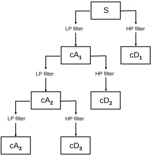
Unlike Fourier analysis which can only be used to extract information on the frequency content of a signal, wavelet analysis can be used to investigate both time and frequency characteristics. Like Fourier analysis, wavelet analysis can be formulated via a continuous or discrete wavelet transform. Previous work on activity monitoring has employed the discrete wavelet transform (DWT), therefore our discussion will focus on this method. The discrete wavelet transform is normally implemented using the filter bank interpretation. In this approach the original signal is successively decomposed into separate low and high pass filtered signals, referred to as approximation and detail coefficients respectively.
FIGURES 2 AND 3 ABOUT HERE
If we consider the original signal (S) with maximum frequency fmaxthen the first approximation coefficient
(cA1) is obtained by passing the original signal through a low pass filter with passband [0, fmax/2]. Similarly,
to obtain the first detail coefficient (cD1), the original signal is filtered with a high pass filter with passband
[fmax /2, fmax]. The wavelet coefficients cA1 and cD1 represent the first level of wavelet decomposition.
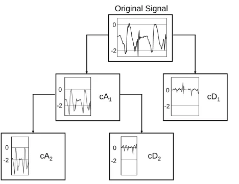
coefficient from the previous level. This process is illustrated schematically in Figure 2 and on an example signal in Figure 3. At each level of wavelet decomposition the filtered signal is downsampled by a factor of two in order to produce the approximation and detail coefficients. Thus, if the original signal contains N
samples, then the first approximation and detail coefficients will be of length N/2. Similarly, the length of the approximation and detail coefficients at the second level of decomposition will be N/4. This process of subsampling reduces the number of time samples and effectively decreases time resolution. This successive halving of the frequency band with each level of wavelet decomposition increases frequency resolution. This compromise between time and frequency resolution allows the wavelet transform to provide good frequency resolution at low frequencies (higher levels of decomposition) but also better time resolution at higher frequencies (lower levels of decomposition).
Wavelet analysis allows a body-worn sensor signal to be decomposed into a number of individual coefficients, each of which contains data on a specific frequency band. As these coefficients characterise the original signal along its entire length, they contain information on temporal changes in frequency content. Thus unlike, Fourier analysis, wavelet techniques can be used to analyse and characterise non-stationary signals (those in which frequency context changes over time). There are a number of different types of DWT, such as the Haar, Daubachies and Coiflets transform, the difference between these different transforms being in the filters used for decomposition. For more complete description of the fundamental principles underlying wavelets, the reader is directed to Rioul and Vetterli [62], walker [57] and Graps [63].
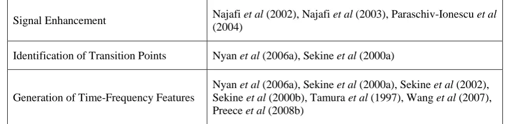
schemes (Section 5.1) which use heuristic features to characterise some aspect of movement or posture (Najafi et al 2003; Paraschiv-Ionescu et al 2004).
TABLE 1 ABOUT HERE
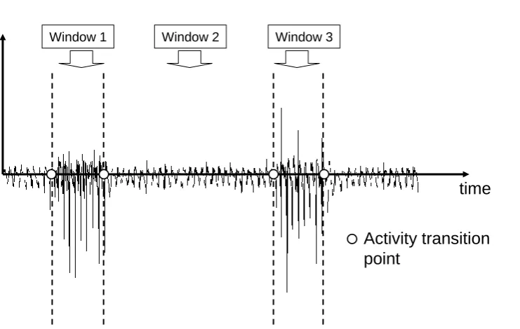
Wavelet analysis can be used to identity the points in a body-worn sensor signal at which there is a change in the frequency content. Recent work by Sekine et al (2000a) and Nyan et al (2006a) demonstrated that, by identifying such points, it was possible to determine the transition times between three different types of gait. Sekine et al (2000a) used wavelet packet analysis to decompose the signal and then reconstructed a low frequency version of the original signal. With wavelet packet analysis, the detail coefficients (Figure 2) are also split into approximation and detail signals (Mallat 1999). Manually set thresholds were then applied to the original signal to identify changes in frequency content and thus walking pattern. Rather than reconstructing the original signal, Nyan et al (2006a) determined transitions from a correlation signal. This was obtained by multiplying the wavelet approximation signals at the two highest levels of decomposition. The technique of multiplying wavelet coefficients, known as direct spatial correlation, can be used to sharpen major signal edges while suppressing noise (Xu et al 1994). By comparing a rescaled version of the correlation signal with the approximation signal at the largest scale, they were able to determine the points at which the walking pattern changed. Both Sekine et al (2000a) and Nyan et al (2006a) specified activity-defined windows from the previously determined transition points. Classification was then performed separately for each window.
In both these studies the wavelet parameters were shown to be significantly different between the three activities.
A number of studies have demonstrated the possibility of using wavelet analysis in activity classification. For example, Sekine et al (2000a; 2000b) and Nyan et al (2006a) used wavelet parameters based on the sum of the squares or RMS of specific detail coefficients as input to threshold-based classification algorithms.. In a similar spirit Wang et al (2007) derived wavelet parameters using simple statistical measures, such as SD and RMS, of specific approximation and detail coefficients which were subsequently used as input to a Neural Network. In a recent paper by Preece et al (2008b) the performance of a number of wavelet-based sets was compared to previously used time- and frequency-domain features for the classification of eight different activities. In general, the wavelet features tended to be outperformed by the time- and frequency-domain features. This result suggest that, although wavelet analysis can be used to analyse non-stationary signals, it may not be the most effective method for characterising short windows of sensor data over which there is minimal variation in frequency content.
4.5 Feature selection methods
Different individuals may perform the same movement in a variety of different ways. This can lead to substantial variability in the features derived from body fixed sensor data (Heinz et al 2003). Hence, for effective classification, it is important to identify a set of features which have high discriminative ability (Kiani et al 1997). A good feature set should show little variation between repetitions of the same movements and across different subjects but should vary considerably between different activities. Furthermore, it is important to minimise any redundancy between features as this can result in unnecessarily increased computational demands and, also, reduced accuracy with some classification methods (Duda et al
2001; Theodoridis and Koutroumbas 2006).
activities and showed little overlap were selected for subsequent analysis. In their study of six daily activities, Maurer et al (2006) used correlation-based feature selection. With this approach optimal features are defined as those which exhibit high within-class but low between-class correlations.Another method for feature selection is a forward-backward search in which features are sequentially added and removed from a larger set. Optimal features are identified depending on the resulting classification accuracies for each feature subset. This approach was used by Pirttikangas et al (2006) to identify the best sensors/features for the classification 17 different activities
Huynh and Schiele (2005) compared a range of different acceleration-derived features, including mean, variance, spectral energy and FFT coefficients. The acquired data patterns were subjected to k-means clustering in the feature space. Clustering is a method to locate concentrations of data points well separated from each other, and to extract the cluster centres that represent those patterns. Huynh and Schiele (2005) measured the cluster homogeneity to assess whether individual activities tended to cluster together. In order to automatically recognise activities, they labelled the centroid of each cluster with the dominating activity, and they used a nearest neighbour rule to assign a class to a new pattern (Section 5.4). Their analysis showed that, in general, FFT coefficients were best for differentiating between dynamic activities, but they were unable to identify single FFT coefficients which performed best for all activities.
4.6 Dimensionality reduction methods
As an alternative to selecting a subset of the existing features, it is often possible to combine the original features to define a new set of variables. There are two benefits associated with such a procedure. Firstly, the often unnecessarily large numbers of features, resulting from many sensors, can be reduced. Secondly, the new reduced variables frequently have better discriminative ability for classification problems. One of the most common techniques for reduction is Principal Component Analysis (PCA) (Chau 2001a; Duda et al
Theodoridis and Koutroumbas 2006) extends PCA to non-Gaussian data, where the sought directions produce variables that are statistically independent from each other. The variables are still reduced as in PCA, but a general linear transformation, as opposed to the rotation of PCA, is performed and often enhances the classification ability of many algorithms.
Previous authors have applied dimensionality reduction methods to different aspects of activity classification problems. For example, Mantyjarvi et al (2001) preprocessed data from two tri-axial accelerometers using PCA and ICA, and used this as input to a Wavelet-based feature generation technique. For a five-activity problem, high levels of classification accuracy (83-90%) were obtained using a neural network classifier. Following similar principles Krause et al (2003) used PCA to reduce the high dimensionality of a 128 FFT feature set (Section 5.11). Using a slightly different approach Huynh and Schiele (2006b) developed an algorithm based on multiple eigenspaces. This technique extends PCA in the sense that it uses multiple spaces spanned by subsets of the PCA eigenvectors. Using this method Huynh and Schiele (2006b) were able to decipher structure in accelerometer data without any user annotation or information on the activities involved. In subsequent work Huynh and Schiele (2006a) applied this approach to data collected by Kern et al (2003) using tri-axial accelerometers distributed across the body. The multiple eigenspaces algorithm provided a low-dimensional description of original sensor data which was then used as input to an SVM (Section 5.6) classification algorithm.
5 Classification Schemes
in order to ‘train’ the classification algorithm. Once the training phase is complete the classifier is able to assign an activity label to an unknown window of sensor data. With unsupervised approaches no activity labels are required for the training dataset. Instead, all the sensor data is passed to the algorithm which automatically identifies a number of states or data clusters, each of which may correspond to a particular activity.
Within the field of activity classification, the classical Cross-Validation (CV) (Duda et al 2001) can be adapted to evaluate the accuracy of the system in two ways: between-subject and within-subject evaluation. In the former case, the classifier is first trained with data from all subjects except a few and then tested with data from the excluded subjects. The accuracy is then calculated as the proportion of correctly classified windows of data across all activities. The process of excluding some subjects and performing a train-test cycle is repeated until all subjects have participated in the testing datasets. The finally overall accuracy is then calculated as the average accuracy across all train-test cycles. When one subject is used for the testing, for a number of cycles equal to the number of subjects, this is called leave-one-subject-out CV. For within-subject evaluation, training is performed using a portion of windows for a specific within-subject, while testing takes place with the remaining samples of the same subject. This process is then repeated, each time using a different portion of the subject samples for testing. The overall accuracy is determined from the average of all the cycles for all available subjects.
Although an overall accuracy is often provided, more detailed views of the classifier’s performance can be given through sensitivity and specificity. These are calculated separately for each activity by determining whether each data window in the test dataset has been identified as the correct activity or not. Sensitivity represents the ability of the classifier to select instances of a certain activity class, whereas specificity represents the true negative rates of an activity. These measures are based on the analysis of the confusion matrix, which summarises the predicted and actual instances for each class.
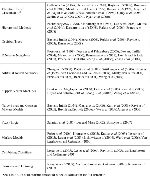
section, 5.11.Finally, in Section 5.12, we present an overview of the different classification techniques. Table 2 lists the different classification methods along with corresponding published studies.
TABLE 2 ABOUT HERE
5.1 Threshold-based classification
With threshold-based classification a derived feature is simply compared to a predetermined threshold to determine whether a particular activity is being performed. This approach has been used successfully to differentiate between static postures, such as standing, sitting and lying, using angles derived from accelerometers placed on combinations of the pelvis/trunk (Boyle et al 2006; Culhane et al 2004; Uiterwaal
et al 1998), lower limb segments (Busser et al 1997; Bussmann et al 1998c; Culhane et al 2004; Makikawa and Iizumi 1995) and chest (Aminian et al 1999b; Najafi et al 2003). Threshold-based classification has also been used successfully to identify postural transitions using data on the change in segmental angles derived from either accelerometers (Najafi et al 2003) or gyroscopes (Najafi et al 2002; Najafi et al 2003). These algorithms are typically sensitive to the exact choice of threshold angle (Najafi et al 2003). Therefore, as an alternative, Najafi (Najafi et al 2003) proposed a simple kinematic model in which vertical displacement of the chest sensor was estimated from double integration of the acceleration signal.
It is common to differentiate between static postures and dynamic activity by using a feature which quantifies variation in the acceleration signal (Section 4.1) (Mathie et al 2003; Maxwell 2002; Veltink et al
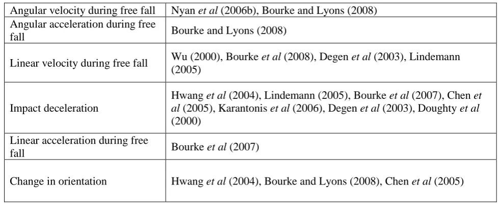
Threshold-based classification has been successfully applied to the detection of falls. A fall can be considered an extreme instance of a postural transition. As explained in Section 4.1 a range of different characteristics have been used to develop heuristic features which are then used in threshold-based classification schemes. This range of different characteristics has been summarised in Table 3.
TABLE 3 ABOUT HERE
Both Nyan et al (2006b) and Bourke and Lyons (2008) studied angular velocity and angular acceleration characteristics during a fall. They found significantly larger values during a fall than in everyday activities,, demonstrating the potential for accurate falls identification. Wu (2000) studied the horizontal and vertical velocity characteristics of falls using an optical motion capture system and showed that trunk vertical velocities associated with falls were 2-3 times those of everyday activities. More recently, Bourke et al
(2008) used an inertial measurement unit (accelerometer and gyroscope) to measure vertical velocity and then applied a threshold of 1.3 ms-1 to identify falls with 100% accuracy. Other researchers have obtained an
estimate of linear velocity by directly integrating the signal from an accelerometer (Degen et al 2003; Lindemann et al 2005) and again applied simple thresholds to identify falls.
The most common characteristic used to identify the presence of a fall is the rapid deceleration which occurs as the faller contacts the ground (Chen et al 2005). Different thresholds have been reported for different accelerometer placements (Doughty et al 2000). Thresholds of 6g, 3.5g and 2.7g have been reported for accelerometers mounted at the ear, trunk and thigh, respectively (Lindemann et al 2005; Bourke et al 2007). Bourke et al (2007) further compared the accuracy of fall detection using two threshold rules, one applied to the impact deceleration and the other to the acceleration during free fall. Their results showed the impact deceleration to be a more effective means of identifying falls from everyday activities, with 100% specificity compared to 91% specificity for free fall acceleration.
Bourke and Lyons (2008) combined three threshold-based rules using angular velocity, angular acceleration and orientation and demonstrated that falls could be differentiated from everyday activities with an 100% accuracy. Other studies have combined acceleration thresholds with a measure of change in orientation (Chen et al 2005; Hwang et al 2004), again reporting high levels of accuracy. After detection using threshold-based methods, the occurrence of a fall is often confirmed by checking for a period of inactivity (Doughty et al 2000). For example Hwang et al (2004) suggested a period of 10 seconds and Karantonis (2006) a period of 60 seconds.
5.2 Hierarchical methods
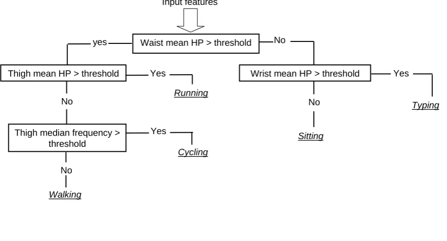
To implement a hierarchical classification scheme, a binary decision structure is constructed which consists of a number of consecutive nodes. At each node a binary decision is made depending on the input features. This decision results in either a definite classification being made or in a transition to another node, where further differentiation between activities is performed. The exact nature and parameters of the decision made at each node is obtained via manual inspection and analysis of the training data, which means that this approach is very time consuming. An example decision structure is illustrated in Figure 4. Although this example uses only simple threshold-based rules, it is possible to base the node decision on any mathematical operation.
FIGURE 4 ABOUT HERE
More recently, Parkka et al (2006) applied a threshold-based hierarchical classification scheme to differentiate between eight different dynamic activities (Table 4). In a follow-on study, Ermes et al (2008) investigated the same set of activities but also included football and compared the performance of the hierarchical approach to other standard classification schemes (Table 4). They also developed a hybrid classification scheme in which each node of the hierarchical structure consisted of an artificial neural network. When all data was used for evaluation purposes, this hybrid model was shown to outperform both an artificial neural network and the hierarchical classifier.
The hierarchical approach was also used by Mathie et al (2004a) in a study using a single tri-axial accelerometer. In addition to threshold-based rules they used probabilistic methods and signal morphology techniques to make the classification decision at each node. They demonstrated that this approach could be used to differentiate between a large range of postures, activities and postural transitions across 26 healthy subjects. Furthermore, by including an additional node which identified abnormal peaks in the accelerometer signal they could identify possible falls. A simplified and computationally efficient version of this algorithm was later developed by Karantonis et al (2006) which used only simple threshold-based decisions at each node and demonstrated the potential of their hierarchical approach for real-time fall detection.
5.3 Decision trees
The decision tree approach is similar to hierarchical classification. However, rather than the decision structure being constructed manually by the user, rigorous algorithms exist to automate the process and create a compact set of rules (Duda et al 2001; Webb 2002). These algorithms work by examining the discriminatory ability of the features one at a time to create a set of rules which ultimately leads to a complete classification system. For further details of the different types of decision tree algorithms the reader is directed to Godfrey et al (2008), Quinlan (1996) and Duda (2001).
Decision trees have been applied to a wide range of classification problems (Ermes et al 2008; Parkka et al
sensors, they obtained an accuracy of 86%. However, additional analysis showed an accuracy reduction of only 3% if only data from a thigh and wrist sensor was used. Maurer et al (2006) investigated the performance of different features and classifiers in the recognition of six different activities (Table 4). The long term goal of their research was to develop a real-time classification algorithm using data from only one wrist-mounted sensor. Ultimately, they used time-domain features which can be calculated with less computational power than frequency-domain features, as input to their decision tree classifier.
5.4 k-Nearest Neighbour
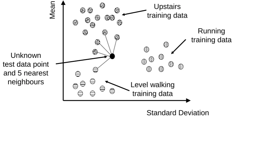
With a k-Nearest Neighbour (kNN) classification scheme (Duda et al 2001; Theodoridis and Koutroumbas 2006), a multi-dimensional feature space is constructed, in which each dimension corresponds to a different feature. The feature space is first populated with all training data points, each of which corresponds to a particular activity. Unknown windows of sensor data are represented in the features space and the k nearest points (or neighbours) of training data identified. Classification is then determined by the majority of the k nearest neighbours which correspond to a given activity. The value of k typically varies from 1 to a small percentage of the training data, and is selected using trial and error, or ideally using cross-validation procedures. Figure 5 illustrates the k-nearest neighbour approach, where a 2D feature space has been constructed. In general the kNN approach can be applied to any number of dimensions.
FIGURE 5 ABOUT HERE
A similar approach was used by Bussmann et al (2001) who defined a 21 dimensional feature space using data derived features from three different accelerometers,. Rather than applying the standard kNN approach, they used training data for each activity to specify a maximum and minimum value along each axis. This effectively defined a volume corresponding to each activity within the feature space. For an unknown window of activity data, classification was determined by the closest activity volume within the feature space. With this approach they were able to identify a wide range of movements and postures with good levels of accuracy (89-93%). More recently the kNN approach has been compared to other classification schemes (Bao and Intille 2004; Maurer et al 2006) (Table 4) and used as part of an algorithm for comparing different features for activity classification (Huynh and Schiele 2005; Preece et al 2008b).
Zhang et al (2006c) used the kNN approach to differentiate between falls and everyday activities. With their classification scheme, a window of accelerometer data was identified immediately before each period of motionless. Non-negative matrix factorisation was then used to extract features from the sensor data which were used as input to the classifier. This factorisation is used to decompose the data matrix into a vector basis matrix and a coefficient matrix, under certain constraints, so that new features can be obtained. The results showed that, in most scenarios, it was possible to differentiate between falls and common activities with >95% accuracy.
5.5 Artificial neural networks
An artificial neural network (ANN) can be likened to a flexible mathematical function configured to represent complex relationships between its inputs (independent variables) and outputs (dependent variables). The ANN is initially presented with a set of training data and some form of optimisation process is employed to enable known outputs to be predicted for a given set of inputs. Once trained the ANN can then be used to obtain the outputs for any set of inputs. In the field of activity classification the inputs are normally features derived from sensor data with the outputs being the different classes of activities. As well as being used for classification problems, ANNs can also be used to estimate continuously varying outputs from a set of input variables (Aminian et al 1995; Findlow et al 2008; Goulermas et al 2005; Herren et al
Ohno-Machado and Rowland 1999). For further background information the reader is directed to Haykin (1999) and Bishop (1999).
One of the most common ANNs is referred to as a multi-layer feedforward neural network or multilayer perceptron (MLP) (Bishop 1999; Haykin 1999). This consists of inputs and outputs which are interconnected via special nodes, distributed in so-called ‘hidden’ layers. The flow of information through the network is controlled by the weighting of the links between the nodes and the transfer function within each node. This type of network is trained by iteratively optimising the weights in order to accurately produce the desired training outputs from the corresponding inputs. Zhang et al (2005) used this approach to classify a four-activity problem using data from pressure sensitive insoles. By using features derived via parameterising the ground reaction force as input to the ANN, Zhang et al (2005) were able to accurately (>97%) identify the type of activity as well as predict the speed of walking and running. Other studies which have used an MLP include Baek et al (2004), Mantyjarvi et al (2001) and Wang et al (2007) with a further three studies (Ermes
et al 2008; Parkka et al 2006; Pirttikangas et al 2006) comparing the accuracies obtained using an MLP to those obtained with other classification approaches (Table 4) .
An alterative to the feedforward ANN is the probabilistic neural network (Specht 1990). Unlike most ANNs which require an extensive training period, this type of network enables classification to be rapidly performed using example patterns stored in memory (Specht 1990). Kiani et al (1998) employed this approach, training their ANN using template waveform patterns for each activity, rather than using features derived from sensor signals. Although their classification scheme was straightforward to implement, an individually designed network was required for each subject.
tilt switches did not perform as well as the accelerometer-based approach, relatively good classification accuracy was demonstrated for a range of daily activities, especially static postures.
5.6 Support Vector Machines
Support Vector Machines (SVMs) (Cristianini and Shawe-Taylor 2000; Vapink 1998) constitute a popular machine learning method which is based on finding optimal separating decision hyperplanes between classes with the maximum margin between patterns of each class. Additionally, by using the so-called kernel functions, they can project the data from the original feature space they lie in, to another higher dimensional space. In this way, a linear separation in the new space becomes equivalent to a non-linear classification in the original space. An optimisation technique is used to find the optimal separating hyperplanes that perform the required classifications.
SVMs have only been applied in a small number of activity classification studies. Huynh and Schiele (2006a) combined a multiple eigenspaces approach (Section 4.6) with SVM and were able to consistently outperform a Naive Bayes approach even with very small amounts of training data. In another study, Krause
et al (2005) used an SVM and showed better performance of frequency-domain over time-domain features for the recognition of eight daily activities.
dropped to 84% when they attempted to identify falls from other high intensity activities, such as running and jumping.
5.7 Naive Bayes and Gaussian mixture models
The Bayesian classifier is based on the estimated conditional probabilities or likelihoods of the signal patterns available from each activity class. Given such likelihoods, the probability of a new unknown pattern having been generated by a specific activity can be estimated directly With a Naive Bayes classifier the input features are assumed to be independent of each other. With this assumption it is possible to express the likelihood function for each activity, as the product of n simple probability density functions, where n is the number of features. These functions are typically expressed as one-dimensional Normal distributions. Although the assumption of feature independence is often violated, the Bayesian approach is popular due to its simplicity and ease of implementation. A more general version of the Naive Bayesian is Discriminant Analysis, where cross-correlations between features are taken into account. For further details the reader is directed to (Duda et al 2001; Theodoridis and Koutroumbas 2006).
Mixed results have been reported when the Bayesian approach to activity classification has been compared to other methods (Table 4). For example, Maurer et al (2006) and Ravi et al (2005) found this approach to either outperform or match the classification accuracy of other methods, whereas Bao and Intille (2004) found low levels of classification accuracy. Bao and Intille (2004) suggested that the reason for this poor performance may have been the questionable assumptions that acceleration features can be considered conditionally independent and modelled by a normal distribution. Other studies which have used the Bayesian approach are Huynh and Schiele (2006a), Kern et al (2003) and Wu et al (2007). In this latter study Wu et al (2007) developed a generic classification method which could discern when to use available sensors to achieve a specified level of certainty. They demonstrated their approach through a case study in which they distinguished between different types of limp using accelerometers and knee-angle sensors.
assumed to be of unknown shape and functional form and thus approximated by a weighted mixture of Gaussian functions. The weights and the parameters (centres and covariances) of the mixture components are calculated using the expectation-maximisation (EM) algorithm. Allen et al (2006) employed this approach using time-domain features to construct separate GMMs for a number of movements/postures. To train the GMMs and calculate the parameters they used an approach similar to EM but which employed a statistical estimate proposed in the field speech recognition. Classification of test data was achieved by selecting the GMM (activity) with the highest probability of having produced that particular set of features. Allen et al
(2006) showed that, provided subject-specific training was used, the GMM outperformed a hierarchical classifier (Table 4).
5.8 Fuzzy Logic
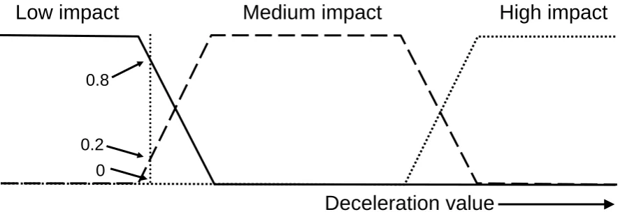
Fuzzy logic is derived from fuzzy set theory and uses reasoning which is approximate rather than precisely defined. It allows mapping from a set of inputs to one or more outputs via a set of if-then statements called rules. For an activity classification problem, features derived from body-worn sensor signals constitute the inputs, with the outputs being fuzzy truths corresponding to each class of activity. Information flows through a fuzzy system via a number of steps. Firstly, the inputs (or features) are assigned membership to fuzzy sets via appropriate membership functions. In contrast to classical set theory in which a data point’s membership is either in or out, by allowing the membership function to range between 0 and 1 fuzzy set theory permits partial membership in multiple sets,. Figure 6 illustrates example membership functions which could be used to describe the size of an impact deceleration in terms of three sets: low, medium or high impact. As an example, a dotted vertical line has been used to specify a deceleration value which has the membership function values of 0, 0.2 and 0.8 for high, medium and low respectively. Once each input has been assigned membership of a fuzzy class, the rules can be applied to produce a corresponding output. For an activity classification problem, this output is a membership value, or fuzzy truth, ranging from 0 to 1 for each class of activity. The classification result is then normally taken to be the activity with the maximum fuzzy truth.
decision tree classification schemes. Despite this, fuzzy logic has only been applied to a limited number of activity classification problems. Lee and Mase (2002) applied this approach, first using simple heuristic features to identify different static postures, and then using the fuzzy classifier to differentiate between different movements. They defined membership functions in terms of the standard deviations of the sensor signals and the short-term change in orientations, calculated from the gyroscope signal. By using a set of rules based around the min operation (the fuzzy equivalent of AND), Lee and Mase (2002) were able distinguish between different gaits with good accuracy (>90%).
The Mamdani fuzzy inference method is one of the most common techniques for developing a fuzzy logic classifier. With this approach it is possible to specify certain membership functions and then to develop a set of rules which allows the training inputs (features) to be mapped to the training outputs (activity classes). Salarian et al (2007) used this method as part of a three-stage activity classification scheme. This scheme first used a statistical classifier to identify sit-to-stand and stand-to-sit transitions and then employed a threshold-based approach to identify periods of walking and lying. Finally, a fuzzy classifier was used to identify periods of sitting and standing. This classifier was developed using membership functions constructed from a knowledge of activity states before and after period of interest. Classification accuracies obtained using this approach were shown to be better than those obtained using simple threshold rules (Najafi et al 2002).
Boissy et al (2007) used Mamdani’s fuzzy inference to identify falls. Data from a tri-axial accelerometer were used as input to a fuzzy classifier and the amplitude of each acceleration component used to determine membership values for the classes: low, medium and high (Figure 6). A total of 27 rules were used to produce the output, which was expressed in terms of a three-class membership function (‘no’, ‘maybe’ and ‘yes’) representing the occurrence of a fall. The value of this output function was then combined with knowledge of body orientation using conventional Boolean logic to determine whether a fall had occurred. By collecting a large dataset of fall and non-fall events from 10 subjects they were able to demonstrate average fall detection accuracies ranging between 86 and 93%, depending on sensor location.
For certain classification problems, some transitions between activities are more likely to occur than others. For example, it is highly unlikely that an individual would sit down directly after descending stairs, but would be likely to start walking. A Markov chain is a discrete time stochastic process in which each activity is represented as a different state. Markov chains can be used to represent the likelihood of transitions between different activities.
A HMM is similar to the Markov chain, but the state of the model at any given time is unknown (or hidden) and can only be determined from observable parameters which depend on the state. By contrast to the Markov chain, the HMM can be used directly for activity classification problems. The observable parameters are the features derived from body-worn sensor data, with the states corresponding to the different activities. Unlike a Markov Chain, states in a HMM can correspond to more than one activity. As with previous classification techniques, a HMM is first trained using example data. Once trained, it can then be used to determine the most likely sequence of state transitions (and thus activities) which could have resulted from an observed sequence of features. HMMs are trained by determining state transitions along with the probabilities that each possible set of observations (features) will be observed for a given state. These probabilities are obtained using the Baum-Welch algorithm (McLachilan and Peel 2000). In activity classification studies, HMMs have been used as a single classifier (Pober et al 2006) and as part of a two-stage classification scheme (Lester et al 2006; Lester et al 2005; Ward et al 2006). They have the advantage over other classifiers that they can be used to model any constraints that are imposed on the sequence in which activities can occur.
the different workshop activities with an accuracy of 74-78% with subject-specific training (Ward et al
2006).
Lester et al (2006; 2005) used the HMM formulation as part of a two-layer classification for differentiating between a range of daily activities. The output probabilities from a large number of static binary classifiers (Section 5.10) were used as input to the HMM. The addition of the HMM layer allowed the classifier to account for sequence constraints thereby increasing the accuracy of activity recognition by as much as 10-15% (Lester et al 2006). It also had the effect of smoothing out sporadic errors which occurred when the simple static classifiers were used alone, ensuring temporal smoothness in the final activity profile.
For applications in which the aim is not to determine a continuous activity profile from a set of observed features, but simply to know transition probabilities to subsequent activities a simple Markov chain can be used. Krause et al (2005) used Markov chains to determine the optimal strategy for selectively sampling sensor data, demonstrating the potential to reduce power consumption. Specifically, for activities which were known to have short duration, a short sampling interval was selected, whereas for longer duration activities, the sampling interval was increased. Markov chains have also been used as part of unsupervised learning algorithms (Krause et al 2003; van Laerhoven and Cakmakci 2000), for details see Section 5.11.
5.10 Combining Different Classifiers
AdaBoost is a type of adaptive boosting that incrementally trains classifiers by suitably increasing the pattern weights to favour the misclassified data. Thus, it combines multiple weak classifiers to create a single more powerful one and has been used by Lester et al (2006; 2005) and van Laerhoven and Gellersen (2004). Lester et al (2006; 2005) studied 10 common daily activities deriving a large number of statistical and frequency-domain features from a range of sensors. They then constructed a set of weak binary classifiers, each of which accepted only a single feature as input and obtained a classification result from a weighted combination of the weak classifiers. They compared the performance of two different weak classifiers: a discriminative decision-stump (a binary decision tree classifier constrained to the use of a single feature) and a generative Naive Bayes model (Section 5.7) and found the Bayesian approach to perform best. Classification accuracy was then improved by using the output from the weak classifiers as input to a HMM (Section 5.9).
5.11 Unsupervised learning
Van Laerhoven and Cakmakci (2000) were the first to demonstrate the potential of unsupervised learning techniques in activity monitoring. They defined a feature space from a number of simple time-domain features obtained from two thigh-mounted accelerometers. A Kohonen self-organising feature map (SOM) was then used to identify localised patterns within the feature space. A SOM can be considered an array of discrete nodes or neurons, used to store projections of the original data to a much lower dimensional feature space. It does so by recognising and maintaining the groupings and proximity characteristics of the data in the original space. During unsupervised learning, each original pattern is projected onto the network topology and the strongest pattern activation is used to update the weights in the corresponding neighbourhoods. Through this process, the clusters and patterns of points within the original high dimensional feature space are identified and mapped to well-defined regions of the two-dimensional SOM. Once the original data has been grouped in this way it can be labelled with minimal user input and then a supervised classification layer added to recognise unknown windows of sensor data.
After associating specific regions of their SOM with one of seven activities Van Laerhoven and Cakmakci (2000) added a supervised layer which comprised of a kNN classifier and a Markov chain. Unknown windows of sensor data were assigned a potential label via projection onto the SOM after which the kNN method was used to locate the closest activity cluster. Finally the transition probabilities, modelled by the Markov chain, were used to determine whether a particular transition was likely and the classification result modified accordingly.
Unsupervised approaches can be used to identify unusual events from sensor data containing a range of repeated activities. This could be of value for a fall detection system, where there is typically no available training data (sensor outputs during a fall). Recently Nguyen et al (2007) presented a preliminary study demonstrating the potential of unsupervised clustering for the recognition of both usual and unusual events. For their study, they used data from a waist-mounted accelerometer as input to an algorithm which combined Hidden Markov Models and Gaussian Mixture Models to perform data segmentation and clustering without prior knowledge. Each particular activity was represented by a HMM whose density function was estimated using a Gaussian Mixture Model. They investigated the degree to which similar activities clustered together and showed that optimal results were obtained using ‘raw features’ in comparison to other time-domain features. Although their study was carried out on single subject, they demonstrated the potential for an unsupervised fall detection system. Future work is required to better understand the potential of this approach.
5.12 Overview of machine learning classification techniques
Almost all previously published activity classification studies differ in the type and number of activities and in the location, type and number of body fixed sensors. Furthermore, there is considerable variation in the number and type of features which are derived from the sensor signals. This is the case, both for studies investigating a range of normal activities and those concerned with the identification of falls from everyday activities. The variability in activities, sensors and features means that it is not possible to directly compare classification accuracies between different studies. However, a number of studies have compared the performance of two or more classifiers using exactly the same set of input features and therefore allow us to gain some insight into the relative performance of individual classifiers. These studies are summarised in Table 4.
classifiers. For example, Parkka et al (2006) studied eight activities and found that maximal classification accuracy could be obtained with a decision tree classifier. In a subsequent study of a similar set of activities, performance of the decision tree classifier was considerably lower, with the best performance from an artificial neural network. Similarly, although two studies (Lester et al 2005; Ravi et al 2005) obtained relatively good performance with a Naive Bayesian classifier, Bao and Intille (2004) found poor performance using this approach.
Taken together the studies summarised in Table 4 may suggest there is no one classifier which performs optimally for a given activity classification problem. However, many of the different techniques have been evaluated using small numbers of subjects. Therefore, there is a need for further studies investigating the relative performance of the range of different classifiers for different activities and sensor features and with large numbers of subjects. For example, techniques such as SVM and Gaussian mixture models show considerable promise but have not been applied to large data sets.. Fuzzy logic and Markov models also have the potential to be of value in future algorithms as they can be implemented as either a single classifier or as part of a hybrid classification algorithm.
The choice of classifier for any given problem will be determined by a number of considerations. As well as accuracy, factors such as ease of development and speed of real-time execution will influence the final choice. The following paragraphs briefly summarise the different techniques, giving a simple overview of the potential advantages and disadvantages of each method.
Classification schemes using the kNN approach can be developed rapidly, are highly versatile and can be used to classify a large range of different activities. However, on-line execution may be slower than decision trees due to the distance evaluation requirements. Similar to the kNN approach, artificial neural networks are a very flexible, powerful approach which have the potential to be used for a range of different classification problems as well as for predicting functional parameters. Although they have demonstrated high levels of accuracy for a number of classification problems (Table 4), they can be slow to train and some types of networks difficult to implement. SVMs are also a very powerful and popular method and, although they have shown significant potential, they have not been applied to many activity monitoring problems. With this approach it is possible to work reliably with difficult and noisy classification datasets, but they may be very slow to train with large datasets and difficult to set their kernel type and kernel parameters.
Naive Bayes classifiers are simple to develop and can be executed rapidly. However, they are based on the weak assumption of feature independence. Although they have been shown to work well on studies with small numbers of subjects, they tend to be outperformed by other classifiers in large studies (Table 4). Gaussian Mixture Models are more powerful than the Naive Bayes method. However, it is often difficult to set the number of mixtures to obtain optimal density functions. Promising results have been obtained using this approach in one study (Allen et al 2006) and further work is required to establish whether it is applicable to other activity classification problems.
Fuzzy logic holds considerable promise for activity classification problems as it enables reasoning with imprecise concepts. Potential disadvantages of this approach are the difficult construction of appropriate membership functions and uniquely interpreting and combining fuzzy rules. A small number of previous studies have demonstrated good classification accuracies using fuzzy logic, particularly in falls detection, but further work is required to determine the full potential of this approach.