Agent Based Fault Detection System for Chemical Processes using Negative Selection Algorithm

(1)

www.astesj.com

Special issue on Advancement in Engineering Technology

Agent Based Fault Detection System for Chemical Processes

using Negative Selection Algorithm

Naoki Kimura*_{, Yuya Takeda, Yoshifumi Tsuge}

Department of Chemical Engineering, Faculty of Engineering, Kyushu University, 819-0395, Japan

A R T I C L E I N F O A B S T R A C T

Article history:

Received: 15 November, 2017 Accepted: 07 January, 2018 Online: 12 March, 2018 Keywords:

Negative selection algorithm Plant alarm system

Fault detection

Recently, the number of industrial accidents of chemical plants has been increasing in Japan. The fault detection system is required to keep chem-ical plant safely. In this study, a fault detection system for a chemchem-ical plants using agent framework and negative selection algorithm was pro-posed. The negative selection algorithm is one of artificial immune sys-tems. The artificial immune system is an imitative mechanism of vital actions to discriminate self/nonself to protect itself. The method was implemented and applied to a complicated chemical plant—which is a boiler plant virtually operated using a dynamic plant simulator. The simulations of fault detection were carried out. And also the results of simulations are presented in this paper.

1 Introduction

This paper is an extension of work originally pre-sented in 2017 6th International Symposium on Ad-vanced Control of Industrial Processes (AdCONIP) [1].

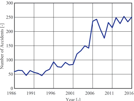
Recently, it has been increasing the accidents of chemical plants. Figure 1 shows the annual numbers of the industrial accidents in Japan (the data is based on the summary of accidents in specified business fa-cilities inside petrochemical complex in Japan, pub-lished by Fire and Disaster Management Agency, Min-istry of Internal Affairs and Communications, Japan, posted on their official web site on May 2017, article in Japanese). The numbers of the industrial accidents in Japan—except accidents caused by earthquakes or tsunami—has been increasing from 45 in 1993 to over 250 in 2016. It is said that the remote causes of the rise of accidents in Japan are mass retirements of skilled engineers, insufficient technical tradition, labor-savings in production lines or plant operations, aged deterioration of productive facilities, or mainte-nance cost reduction in assertive ways. Therefore, ef-fective fault detection system for chemical plants is required. In the general chemical plant operations,

plant alarm systemhas been used to notify the process deviance to operators via warning lights or buzzers in the operation rooms, where the upper and lower thresholds of the measured values or the thresholds of their amounts of changes have been set to the

sen-sors in the chemical plants. However, it is so difficult to determine the adequate values of thresholds (that is ‘alarm setpoint’) that if the alarm setpoints are too small, the alarm floods will be caused, if the setpoints are too large, missed detection of deviation will be caused. And also it is difficult to detect if the plant has normal and regular load fluctuations under both the normal and the abnormal situations. Therefore, a method is required that observes the relationship among several variables to detect faults in a compli-cated system. We focus on the Artificial Immune Sys-tem.

Artificial Immune Systems—which are imitative mechanisms of vital actions of discrimination be-tween self and nonself—have been proposed since 1990s. And a lot of methods have been proposed using various parts of artificial immune systems, for example, pattern recognition by B-cells for fault de-tection in gas lift oil well by Aguilar [2, 3], Natu-ral Killer (NK) immune cells mechanisms by Lauren-tys [4], clonal selection algorithm for maintenance scheduling of power generators by El-sharkh [5], den-dritic cell for failure detection of aircraft by Azzawi [6]. Also lots of applications have been proposed— Wada et al. [7] proposed an fault mode detection method for automotive exhaust gas treatment system, Inomo et al. [8] proposed an failure diagnosis method for water supply network by using immune system. *_{Corresponding Author, [email protected]}

(2)

300

0

2016

1986 1991 1996 2001

Year [-]

2006 2011

50 100 150 200 250

N

u

m

b

er

o

f

A

cc

id

en

ts

[

-]

Figure 1: The annual numbers of the industrial acci-dents in Japan, data from FDMA, Japan.

In this study, we adopt a negative selection algo-rithm to detect faults in a chemical plant. Negative selection algorithm is an imitative method of mecha-nisms of differentiation and maturation, and discrim-ination of normal/abnormal. The algorithm was pro-posed by Forrest in 1994 [13] for the detection of com-puter virus. The negative selection algorithm has been applied to various domains—Dasgupta et al. [9] ap-plied to aircraft fault detection, Gao et .al [10] apap-plied to motor fault detection, Xiong et al. [11] and Prasad et al. [12] applied to fault detection in the Tennessee Eastman process.

In this study, we introduce detectors to detect faults based on the negative selection algorithm. The adopted method of the negative selection algorithm is mentioned in section 2. In order to utilize negative selection algorithm, we designed and implemented an agent based framework of fault detection system, mentioned in section 3. The target chemical process, the simulation conditions and the results are men-tioned in section 4. And the conclusion in section 5.

2 Negative Selection Algorithm

Negative selection algorithm is one of the methods of the artificial immune systems inspired by the vital immune systems. Negative selection algorithm bor-rowed from the mechanism of T-cell generation in thymus. On T-cell generation in vital system, imma-ture T-cells are randomly generated with various im-munological types. And then some of T-cells are elim-inated if they have high affinity with self-antigen to avoid response to “self”. T-cells which are not self-affinitive can be matured to react with foreign antigen to protect itself.

In our system, detectors—correspond to mature T-cells in vital—can detect faults by recognizing the normal operational data of chemical processes which are assumed asselfand the abnormal operational data which are assumed asnonself. In Figure 2(a)–(c), the steps of the generation phase of detectors are

illus-trated. Figure 2(a) illustrates that there are self re-gions in a 2-dimensional process variables space. And the rest area of the variables space arenonself regions. Figure 2(b) illustrates that detector candidates which indicated by plus(+) signs are generated with vari-ous position, where the radius is set as the minimum distance to the self region. In this study, we imple-ment two steps of candidate generation. The first step is a grid-based generation. Place the detector can-didates at every 0.1 of each axis—axis is normalized between [0.0, 1.0]—, therefore 121 (each axis divided into eleven) grid-based candidates are generated. The second step is a semi-randomly generation. Place a detector candidate at random position. Then check whether the new candidate is overlapped on the pre-viously generated candidates. If it overlapped, the new candidate is eliminated in this step, if not, the new candidate is added to the candidates. And then, check the coverage of the detectors. If the coverage is over 90%, candidate generation will be terminated. From Figure 2(b) to (c), the elimination of some can-didates which have affinity with “self” is carried out. Figure 2(c) illustrates that seven valid detectors are re-mained. Then the generation phase is finished.

Self

Nonself

(a) 2-dimensional variable space with

self/nonself regions

(b) Generation of detector candidates

(c) Valid detectors after elimination by self-affinity Detector candidate _{Valid detector}

Figure 2: A schematic diagram of the detectors gener-ation.

In the detection phase, a sample consists of the values of the current process variables—which are to be examined— is plotted into the variable space indi-cated by a ‘star’. If the plotted sample is inside the detection area of at least one detectors, the sample is recognized as “abnormal” (Figure 3(a) ). And if the sample is out of any detection area, the sample is rec-ognized as “normal” (Figure 3(b) ).

(a) A sample which recognized as “abnormal” :plotted

sample

(b) A sample which recognized as “normal”

“Normal” sample “Abnormal” sample

Activated detector

(3)

3 Fault Detection System

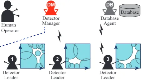
A multiagent framework is adopted to implement a fault detection system using negative selection algo-rithm. In our system, there areDetector Manager, De-tector Leader(s)andDatabase Agentillustrated in Fig-ure 4. Detector Manager is an interface between hu-man operator and the system. Detector Leader(s)have their own variable spaces to detect faults. These vari-able spaces represent relationships between two cer-tain process variables. And there are a lot of detec-tors under the dominion of aDetector Leader. In or-der to avoid missing detection, someDetector Leaders

with variety of combinations of the process variables are required. Database Agent have a database which stores operational database of the target process. All these agents can communicate with other agents via TCP/IP network connection.

Human Operator

Detector Manager

Detector Leader

Database Agent

Database

Detector Leader

Figure 4: A schematic diagram of the detection by de-tectors.

4 Simulations and Results

4.1 Target Process

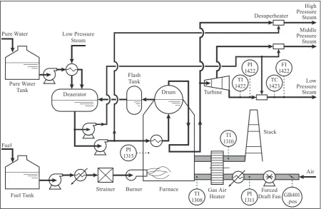
Figure 5 shows a boiler plant which is the target pro-cess of this study. It is an utility plant which supplies three steam headers—high pressure steam (HP), mid-dle pressure steam (MP), and low pressure steam (LP) to the nearby plants by boiling pure water in a fur-nace. Due to the fluctuation of the steam demands from user plants, the boiler plant is always under un-steady operation. Therefore, it is difficult to detect faults by setting up the constant thresholds to some process variables of the boiler plant.

In this study, nine variables were selected from among 120 measured variables in the boiler plant. The selected nine variables are listed in Table 1 and also illustrated in Fig.5. The operational data was obtained by using dynamic plant simulator “Visual Modeler” (Omega Simulation Co., LTD).

4.2 Normal Operational Data

Data of a normal operation—in which the steam demands were stepwise changed without any malfunction—were obtained using the dynamic sim-ulator. The data contain 7200 samples of the

above-mentioned nine process variables and its sampling interval is one second. The trend graphs of PI1422 and TI1422 were indicated in Figure 6. These data were normal operational data which should be rec-ognized as self in the artificial immune system even though the steam demands had increased at time 600 second.

4.3 Abnormal Operational Data

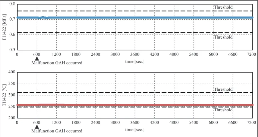
Abnormal operational data with three kinds of as-sumed malfunctions were obtained using the dynamic simulator. Table 2 shows the list of three assumed malfunctions. And Figures 8–10 illustrate the trend graphs of PI1422 and TI1422 when the one of mal-functions was occurred at time 600 second, but with-out any steam demand change during these 7200 sec-onds.

Table 1: Selected nine process variables of the boiler plant.

Variable name Description

FI1422 Flow rate of the second extraction steam from the turbine

PI1422 Pressure of the second extraction steam from the turbine

TI1422 Temperature of the second extraction steam from the turbine

TC1423 Temperature of the low pressure steam from the desuperheater PI1315 Pressure inside the furnace

(upper)

GB401.pos Valve position of the combustion air

PI1311 Pressure of the outlet of the forced draft fan

TI1310 Temperature of the exhaust gas at the gas air heater outlet TI1308 Temperature of the combustion

air at the gas air heater outlet

4.4 Generation of Detectors

(4)

Air Drum

Deaerator

Flash Tank

Furnace

Stack Turbine

Burner Strainer

Fuel

Pure Water Tank

Pure Water Low Pressure Steam

Low Pressure Steam Middle Pressure Steam High Pressure Steam

Forced Draft Fan GB401

.pos TI

1308

PI 1311 TI 1310 PI

1315

TI 1422

FI 1422 PI

1422 TC 1423

Gas Air Heater Fuel Tank

Desuperheater

Figure 5: A schematic diagram of the boiler plant.

time [sec.] 0.5

0 600 1200 1800 2400 3000 3600 4200 4800 5400 6000 6600 7200

0.6 0.7 0.8

P

I1

4

2

[

M

P

a]

time [sec.] 200

0 600 1200 1800 2400 3000 3600 4200 4800 5400 6000 6600 7200

250 350

300 400

T

I1

4

2

[

°

C

]

Steam demand change

(5)

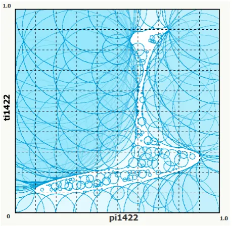
the unpainted parts in Figure 7, and not exist the nor-mal operational data—which correspond “nonself” region—at the painted sky blue parts. The sets of de-tectors were generated for the rest of variable spaces in the same way. The numbers of the detectors in each variable space were from 121 to 316 including both the grid detectors and randomized detectors.

Figure 7: Generated detectors for a 2-dimensional variable space (TI1422 vs. PI1422).

The bold dashed lines in the trend graphs are the maximum and minimum values under the normal op-eration (Figure 6). We can find that it is impossi-ble to detect fault using upper/lower thresholds of variable PI1422 and/or TI1422 when the malfunction BFO or GAH occurred, because the values of PI1422 and TI1422 have not exceeded the ranges under the normal operation. On the other hand, it may possi-ble to detect at time 671 second by lower threshold of TI1422 when the malfunction FDFclose occured at time 600 second. TI1422 also exceeds upper threshold after time 1340 second, shown in Figure 10.

Table 2: Three assumed malfunctions in the boiler plant.

Malfunction ID Description

BFO Burner frame out

GAH Gas air heater rotation failure FDFclose Forced draft fan inlet vane

closure

4.5 Fault Detection using Detectors

Fault detections for the abnormal operational data were carried out. Figure 11 shows an outline of the fault detection in a 2-dimensional variable space con-sisting of TI1422 and PI1422 when malfunction BFO

occurred. The axes and the detectors—indicated by sky blue circles— are the same as Figure 7. The sampling data were plotted by green dots on the 2-dimensional variable space after the normalization for every second serially. The blue dots are the normal operational data and the green dots are the sampling data to be examined by the detectors. These dots are moving in the variable space as time proceeds. If the green dots were placed on the unpainted region, they are recognized as “self”—where the values are similar to the normal operational data. If the green dots were placed over the sky blue region, they are recognized as “nonself”—in other words, a fault was detected in this variable space by detector(s).

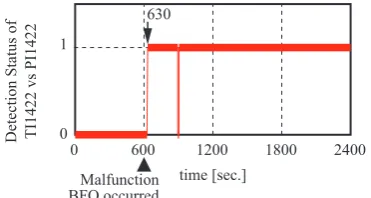
In Figure 11, the painted orange circles indicate activated detectors—which have detected fault. Fig-ure 12 shows the detection status through time. If the value is ‘1’, at least one detector in this variable space detects fault, and if the value is ‘0’, no detec-tor detects fault at that time. The figure shows that the first detection was at time 630 second—which is 30 second after malfunction occurred—, and there are missing between time 897 and 904 second in this vari-able space. The detections using the sets of detectors in the rest of variable spaces were simultaneously car-ried out in the same way. Figure 13 shows the number of variable spaces whose detection status is ‘1’. The figure shows that there are 15 variable spaces detected at time 601 second, 30 variable spaces—which corre-sponds to 80% of 36 variable spaces—detected at time 604 second, and the number does not fall below the 80% after that time. Therefore it can be said that this system can detect malfunction BFO successfully.

Figure 14 shows the outline of the fault detection, Figure 12 shows the detection status through time when malfunction GAH occurred. The figures show that the fault was detected at time 666 second by the detectors. On the other hand, it have not been de-tected after time 1047 second in this variable space TI1422 vs. PI1422. However 16 shows that 21 vari-able spaces—which corresponds to 58% of 36 varivari-able spaces—detected at time 602 second, and the number does not fall below 58% after that time. It can be said that this system can detect malfunction GAH success-fully, although the variable space TI1422 vs. PI1422 could not detect after time 1047 second.

(6)

time [sec.] 0.5

0 600 1200 1800 2400 3000 3600 4200 4800 5400 6000 6600 7200

600 0.6

0.7 0.8

P

I1

4

2

[

M

P

a]

time [sec.] 200

0 600 1200 1800 2400 3000 3600 4200 4800 5400 6000 6600 7200 250

350

300 400

T

I1

4

2

[

°

C

]

Threshold Threshold Threshold Threshold

Malfunction BFO occurred

Figure 8: The trend graphs of PI1422 and TI1422 when malfunction BFO was occurred at time 600 second without steam demands change.

time [sec.] 0.5

0 600 1200 1800 2400 3000 3600 4200 4800 5400 6000 6600 7200

0.6 0.7 0.8

P

I1

4

2

[

M

P

a]

time [sec.] 200

0 600 1200 1800 2400 3000 3600 4200 4800 5400 6000 6600 7200

250 350

300 400

T

I1

4

2

[

°

C

]

Malfunction GAH occurred

(7)

time [sec.] 0.5

0 600 1200 1800 2400 3000 3600 4200 4800 5400 6000 6600 7200

0.6 0.7 0.8

P

I1

4

2

[

M

P

a]

time [sec.] 200

0 600 1200 1800 2400 3000 3600 4200 4800 5400 6000 6600 7200

250 350

300 400

T

I1

4

2

[

°

C

]

Malfunction FDFclose occurred

671 1340

Figure 10: The trend graphs of PI1422 and TI1422 when malfunction FDFclose was occurred at time 600 second without steam demands change.

Figure 11: Fault detection by detectors in a 2-dimensional variable space when malfunction BFO was occurred.

time [sec.] 0

0 600 1200 1800 2400

1

D

et

ec

ti

o

n

S

ta

tu

s

o

f

T

I1

4

2

v

s

P

I1

4

2

630

Figure 12: Detection status of the TI1422 vs. PI1422 variable space when malfunction BFO was occurred.

time [sec.] 0

0 600 1200 1800 2400

40

35

30

25

20

15

10

5

N

u

m

b

er

o

f

d

et

ec

te

d

v

ari

ab

le

s

p

ac

es

Figure 13: The number of detected variable spaces when malfunction BFO was occurred.

(8)

time [sec.] 0

0 600 1200 1800 2400

1 D et ec ti o n S ta tu s o f T I1 4 2 2 v s P I1 4 2 2 Malfunction GAH occurred 666

Figure 15: Detection status of the TI1422 vs. PI1422 variable space when malfunction GAH was occurred.

time [sec.] 0

0 600 1200 1800 2400

40 35 30 25 20 15 10 5 N u m b er o f d et ec te d v ari ab le s p ac es Malfunction GAH occurred

Figure 16: The number of detected variable spaces when malfunction GAH was occurred.

Figure 17: Fault detection by detectors in a 2-dimensional variable space when malfunction FDF-close was occurred.

time [sec.] 0

0 600 1200 1800 2400

1 D et ec ti o n S ta tu s o f T I1 4 2 2 v s P I1 4 2 2 Malfunction FDFclose occurred 630

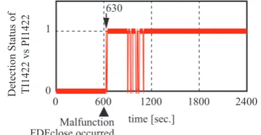
Figure 18: Detection status of the TI1422 vs. PI1422 variable space when malfunction FDFclose was oc-curred.

time [sec.] 0

0 600 1200 1800 2400

40 35 30 25 20 15 10 5 N u m b er o f d et ec te d v ari ab le s p ac es Malfunction FDFclose occurred

Figure 19: The number of detected variable spaces when malfunction FDFclose was occurred.

5 Conclusion

We built up a fault detection system using negative selection algorithms which can focus on the relation-ships between process variables.

References

1. N. Kimura, Y. Takeda, T. Hasegawa, Y. Tsuge, “Agent based fault detection using negative selection algo-rithm for chemical processes” in 2017 6th Interna-tional Symposium on Advanced Control of Indus-trial Processes (AdCONIP), Taipei, Taiwan, 2017. https://doi.org/10.1109/ADCONIP.2017.7983822

2. J. Aguilar, “An artificial immune system for fault detection” Innovations in Applied Artificial Intelligence (17th Interna-tional Conference on Industrial and Engineering Applica-tions of Artificial Intelligence and Expert Systems, IEA/AIE 2004, Lecture Note in Artificial Intelligence), 3029, 219– 228, 2004. https://doi.org/10.1007/978-3-540-24677-0 24 3. M. Araujo, J. Aguilar, H. Aponte, “Fault detection system in

gas lift well based on artificial immune systems” in the Inter-national Joint Conference on Neural Networks, 2003 , 1673– 1677, 2003. https://doi.org/10.1109/IJCNN.2003.1223658 4. C.A. Laurentys R.M. Palhares, W.M. Caminhas, “A novel

artificial immune system for fault behavior detection” Ex-pert Systems with Applications, 38, 6957–6966, 2011. https://doi.org/10.1016/j.eswa.2010.12.019

5. M.Y. El-Sharkh, “Clonal selection algorithm for power generators maintenance scheduling” International Journal of Electrical Power & Energy Systems, 57, 73–78, 2014. https://doi.org/10.1016/j.ijepes.2013.11.051

6. Dia Al Azzawi, Mario G. Perhinschi, Hever Moncayo, Andres Perez, “A dendritic cell mechanism for de-tection, identification, and evaluation of aircraft fail-ures” Control Engineering Practice, 41, 134–148, 2015. https://doi.org/10.1016/j.conengprac.2015.04.010 7. K. Wada, T. Toriu, H. Hama, “Improving the efficiency of

known fault mode detection for immunity-based diagnosis” Transactions of the Institute of Systems, Control and Infor-mation Engineers, 27(2), 59–66, 2014 (article in Japanese with English abstract). https://doi.org/10.5687/iscie.27.59 8. H. Inomo, W. Shiraki, Y. Imai, H. Kanamaru, “Failure

(9)

9. D. Dasgupta, K. KrishnaKumar, D. Wong, M. Berry, “Nega-tive selection algorithm for aircraft fault detection” Artificial Immune Systems (Third International Conference, ICARIS 2004, Lecture Note in Computer Science),3239, 1–13, 2004. https://doi.org/10.1007/978-3-540-30220-9 1

10. X.Z. Gao, H. Xu, X. Wang, K. Zenger, “A study of negative selection algorithm-based motor fault detection and diagno-sis” International Journal of Innovative Computing, Infor-mation and Control,9(2), 875–901, 2013.

11. C. Xiong, Y. Zhao, W. Liu, “Fault detection method based on artificial immune system for complicated pro-cess”, Computational Intelligence (International Confer-ence on Intelligent Computing, ICIC 2006, Lecture

Note in Artificial Intelligence), 4114, 625–630, 2006. https://doi.org/10.1007/11816171 77

12. J. V. Prasad, K. Ghosh, “Negative selection algorithm for monitoring processes with large number of vari-ables”, in 2014 IEEE Conference on Control Ap-plications (CCA), 778–783, Antibes, France, 2014. https://doi.org/10.1109/CCA.2014.6981435