R E S E A R C H
Open Access
The virtual small cells based on UE
positioning: a network densification solution
Thomas Varela Santana
*, Sofía Martínez López and Ana Galindo-Serrano
Abstract
Next wireless generation mobile networks will be composed of a large number of antennas at the base station (BS), which is known as massive multiple input multiple output (MIMO). Thanks to this technology, the BS can focus the energy on a user equipment (UE) or group of UEs to improve their throughput and the network capacity. We call these coverage areas virtual small cells (VSCs). Their main advantage is that they allow increasing the network capacity through a virtual densification, therefore, avoiding the deployment cost of new infrastructure. Identifying the dense traffic areas in real time and providing a good quality of service arises as a key challenge to be addressed. Our work focuses on the interaction between the VSCs and the identification of the dense traffic areas, where a feedback scheme is proposed. This feedback scheme is based on the location of these dense traffic areas provided by our proposed clustering methods. To conduct this research, we propose(i)a VSC architecture and system model with a specific codebook in order to avoid feedback overhead, and(ii)two positioning algorithms in order to determine the hotspots localization. The first positioning algorithm is based on K-means method and is centralized at the BS using Global Positioning System (GPS) coordinates, and the second one is based on cooperative communications using ultra-wideband (UWB) signals in order to avoid the network participation. Finally, simulations of these positioning methods intended for the use of the VSCs are presented. These results show significant improvement compared to already existing methods. Furthermore, these positioning methods highly reduce the feedback since, accordingly to our VSC model, the BS only requires angles information based on the localized hotspots.
Keywords: Massive MIMO, VSC, GPS, UWB, D2D, Positioning, Cluster localization
1 Introduction
Ensuring constantly growing and changing capacity requirements with low infrastructure investment in mobile network is a key challenge for operators. The fourth-generation (4G) considers the introduction of small cells in addition to the base stations (BSs) to deal with dense traffic, as small cells help focusing energy on a given area such as commercial centers, stadiums, etc. Nevertheless, the use of small cells represents high investment for operators as they involves important cap-ital expenditure (CAPEX), i.e. backhaul deployment, site acquisition and also operational expenditure (OPEX), as energy consumption and maintenance [1,2]. This is jus-tified when capacity requirements are stable over time and space.
*Correspondence:[email protected]
Orange Labs, 44 Avenue de la République, 92320 Châtillon, France
Different challenges have been identified in future wire-less communications. An important envisaged require-ment is to provide great service in a crowded network
[3] in a more energy-efficient way. Some examples of
possible scenarios are meeting rooms at certain hours in business buildings, shopping, stadiums, open air fes-tivals, public events, traffic jams, etc. Notice that the occurrence of these scenarios is non-predictable by the operator. The optimal solution, from the infrastructure point of view, could be to adapt the coverage of these unpredictable crowded areas, in terms of time and local-ization, as they are at the origin of dense traffic. The idea is to have an elastic network infrastructure. An example of this, is the Google Loon project [4], where balloons equipped with antenna systems placed at the stratosphere at around 20 km from the surface of the earth and steered using the different wind current layers are used to provide coverage.
In order to avoid the small cells, two-dimensional (2D) large antenna array at the BS named massive multiple input multiple output (MIMO) can be exploited.
Adding more antennas at the BS provides more degree of freedom to the propagation channel between the trans-mitter and the receiver. Due to these degrees of freedom, higher diversity, and higher data rate can be achieved, increasing also the capacity [5–7]. Improvement of energy efficiency in cellular system using an increased num-ber of antennas at the transmitter has been studied and explained in [6] (and references therein). With the use of 2D antenna elements highly directive beams to cover a given area can be created [8]. We call this concept vir-tual small cell (VSC) which consists of highly directive beam working in co-channel that point to cluster esti-mated hotspot, increasing the signal interference noise ratio (SINR) with massive MIMO at the BS and without small cells [9]. Reduction of co-channel interference by using an unlicensed band for the VSCs is proposed in [10]. Security and caching aspects for VSCs have been consid-ered in [11,12] respectively, while ergodic sum-rate has been derived in [13] for VSCs.
The benefits of VSCs compared to three-dimensional (3D) user equipment (UE)-specific beamforming (for massive MIMO) are the following:
• VSC allows to dynamically allocate the radio
resources for each geographical zone according to the dynamic spatial traffic.
• VSCs are transparent for UEs, and can then be used for legacy UEs. On the contrary, UE-specific
beamforming requires UEs that support the number of extend codebooks.
• VSCs are more robust to UE mobility and/or channel variations since the focalization area is wider. If the 3D UE-specific beamforming is narrow, the motion of the UE forces to rapidly update the precoding in order to refocus the energy on the new UE location.
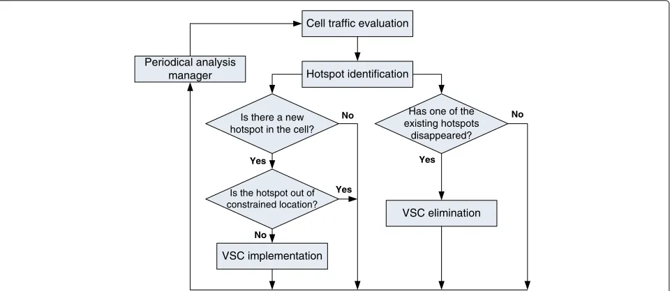
A way to implement the VSCs according to the UEs position is to firstly evaluate the cellular traffic. Secondly, based on the previous cellular traffic analysis, the hotspots of UEs have to be identified. If the detected hotspot is new in the cell, and it respects the constraint location, a highly directive beam will be focused on it, i.e., a VSC is implemented. If hotspots in the database have disap-peared, the associated VSCs are removed. By repeating these previous steps, we obtain a periodical methodology which gives us a general view on when to implement or eliminate the VSCs. This methodology has been presented
in one of our previous works [14] and is summarized in
Fig.1for reading clarity. Concerning the constraint loca-tions, the performance of the VSC can vary depending on its steering point. There are basically two constraints to consider, the VSC steering point should not be too close to the macrocell and should not be at the bore-sight. This
last point is more detailed and represented in Fig. 3 in
Section3.
To implement a VSC, the directive beam is guided thanks to a well design precoder. Precoding is a gen-eralization of beamforming to support multi-stream transmission in multi-antenna wireless communications.
Cell traffic evaluation
Hotspot identification
VSC elimination
VSC implementation Periodical analysis
manager
Is there a new hotspot in the cell?
Has one of the existing hotspots
disappeared?
Is the hotspot out of constrained location?
Yes
No
Yes
Yes No
No
Actually, such a precoder will be chosen depending on a predefined codebook based on specific characteristics of the detected hotspots. These characteristics are the center and the radius of the corresponding hotspot. Depending on operator strategies, several clustering methods have been developed for positioning in fifth-generation (5G) [15] in order to identify such a hotspot. One strategy is to centralize all the information at the BS [14] and another is to identify the hotspots without intervention of the BS by using direct device-to-device (D2D) link between all the
UEs [16]. Both methods need synchronization whether at
the BS or between the UEs [17]. Once a hotspot has been identified, an easy feedback can be performed in order to select the adequate precoder for the beam formation. Smooth feedback information is essential as the large number of antennas made the channel state information (CSI) very important and may cause huge amount of feedback overhead as each antenna needs a feedback from each device. In time division duplexing (TDD) mode, the reciprocity of the downlink and uplink could be used for channel estimation but reciprocity is not available in frequency division duplexing (FDD) mode where uplink and downlink occurs in separated bands. VSC requires less radio overhead for FDD. Indeed, the number of antenna ports for the case of VSC is reduced compared to the case of massive MIMO. In massive MIMO, one different downlink reference signal is needed for each antenna port [18,19]. Therefore, the more antenna ports, the more radio signal overhead is needed at transmission. The feedback of VSC is smaller than the one required for massive MIMO while still able to track changes in the traffic generated by the group of served UEs. Our pro-posed feedback is based on index grouping transmission, where one index is selected from the codebook for each detected hotspot. Once the index information is available at the BS, we can select the adequate precoder and create the VSC.
UE positioning applied to 5G cellular management net-works has been deeply described for different scenarios in [20] and also an architecture improving time response using location for indoor scenarios is presented in [21]. VSCs could be also deployed in indoor scenarios, where nowadays small cells are more commonly used. The home/office scenario is given by the constant and recur-rent human behavior, i.e., switching from houses to offices during the day, to shopping malls and restaurant areas. In this case, the traffic flow is predictive and therefore, oper-ators can know in advance the occurrence of a high traffic demand in a given period of the day at a given location. To fulfill the capacity demand in the crowded areas, operators can previously program the activation and deactivation of VSCs pointing to the identified areas in the adequate peri-ods. Also, giving coverage to deep indoor scenarios could be possible thanks to the high gain achieved by VSCs. This
would substitute the installation of fix femtocells. Also, operators could cover specific floors in business build-ings with VIP users having a punctual meeting or hosting an event.
The contributions of this work are the following:
• Whereas VSC is not a new topic, this paper is the first to provide explicit mathematical description of VSC implementation. In particular, we extend and apply the “one-ring” model to the VSCs and express the corresponding correlation matrix.
• The paper highlights the importance of hotspot location knowledge to efficiently implement VSCs. Indeed, the correlation matrix, number of antennas, codebook, and feedback of the VSC are strongly dependent on the hotspot location.
• Due to this hotspot location dependence, the paper proposes to study and compare hotspots location techniques by firstly generalizing a GPS-based method from [14] and secondly a cooperative UWB method.
• Finally, the paper gives a methodology on how to implement VSC in the real network by comparing different approaches for the steering of VSC.
The rest of this paper is organized as follows: in
Section 3, we start defining the system model and the
architecture of the VSC with SINR evaluation. Section4
extends our model to the case of multi-VSCs by generaliz-ing our system model and by proposgeneraliz-ing a codebook design for feedback scheme. Two methods for group localiza-tion are detailed in Seclocaliza-tion5, one based on BS centralized strategy, and another distributed approach based on direct communication between the devices independently of the
BS. We present the results in Section 6 and end by a
conclusion in Section7.
2 Method section
have been compared in an outdoor LOS environment, and the UWB-based method provides better accuracy results, error estimation smaller than 1 cm in 50% of the cases.
3 Virtual small cell architecture and system model
We consider a specific area where major part of the UEs are localized inside. VSC could be implemented by com-mon BSs, as long as the number of antennas is enough to steer the beam as required [9]. Note that there are two options when using a VSC. The first one is associating a different cell ID to the VSC with respect to the cell. This would correspond to network densification without new equipment deployment. The second one is to use the same cell ID (also same frequencies and mobility management) as that of the cell. In this case, the term VSC could be replaced by beam but would work similarly. This depends
on the actual implementation of VSC, and particularly whether a different cell ID is given or not.
Figure2describes the angles in the horizontal and ver-tical planes that are used for building a VSC. The VSC is hence defined by its steering θtilt and his beamwidth
θ3dB in the vertical plane as presented in Fig.2a. Those two angles can be respectively implemented using simple trigonometric functions:
θtilt= −arctan
h dist
[rad] , (1)
θ3dB=arctan
h dist−r
−arctan
h dist+r
[rad]
(2)
hotspot 3dB
tilt
r
x’
y’
dist
hotspot
(x,y)
tilt 3dB h
dist
r
where dist is the projection in the vertical plane of the distance between the BS and the center of the localized
hotspot, his the height of the BS and ris the hotspot
radius. From the horizontal plane, we can distinguish two other angles,ϕtilt andϕ3dBas represented in Fig.2band expressed using trigonometric functions as follows:
ϕtilt= −arctan
The antenna elements (i.e.,NvandNh antennas in the
vertical and horizontal plane, respectively), used for cre-ating a beam, depends on the angles above. They also depend on the array element distanceλD, whereλis the wavelength factor and on the value 50 that has been given by an antenna expert of our group based on experiments for our topology:
The number of antenna elements at the BS is computed as:
M=Nmc+NVSC (7)
whereNmcare the antenna elements used for the
macro-cell andNVSC=Nv×Nhare the active antenna elements
used to create a beam for the VSCs. This will automatically reduce the CSI feedback overhead because the number of antenna ports for the case of VSC is reduced compared to the case of massive MIMO (NVSC<M).
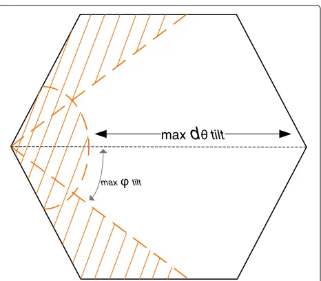
As stated in the introduction, the performance of the VSC can vary depending on its steering point:
• If the VSC steering point is close to the macrocell, the UEs will experience high interference from the macrocell.θtiltwill increase and its projection
distance in the horizontal planedθtiltalso, involving
increased number of antenna elements in the vertical axis, as expressed in (5).
• If the VSC is steering towards the edge of the cell, i.e., if the azimuth angleϕtiltis close from bore-sight, the number of antennas required is higher as shown in (6).
These two location constraints are represented in Fig.3, where dashed areas represent the forbidden regions where VSCs will not be deployed.
Let us consider a BS, whereMantennas elements are
used by the VSC serving K UEs working in FDD over
maxφtilt
max
d
tiltFig. 3Constraint location for VSC in hexagonal cell. This figure represents the constraint location in an hexagonal cell where the VSCs can not be deployed
a Rayleigh-fading channel. For each channelhk ∈ CM,
1 ≤ k ≤ K, a linear precoding is employed at the BS to
support simultaneous downlink transmissions toKUEs.
We callx ∈ CM the linearly precoded signal vector
sub-ject to the transmit power constraintE||x||2 ≤ P. The received signals at theKUEs is represented by the vector y∈CK and can be expressed as
y=HHx+n, (8)
whereH=[h1,. . .,hK] is the downlink channel matrix of
the VSC andn ∼ NC(0,IK)is the Gaussian noise. Also,
the transmitted signal can be written as
x=Ws=
the equally transmitted power allocation and sk ∈ CK
represents the data streams.
Then, the received signal of thekth UE is given by
yk=PkhHkwksk+ K
j=k
PjhHj wjsj+nk, (10)
And the SINR for UEkcan be analytically expressed as
follows:
The work in [9] proposes a comparison between
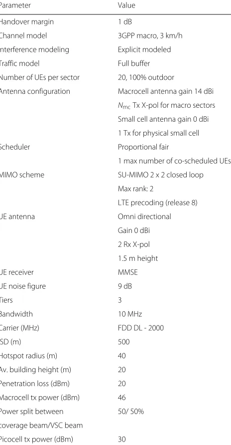
macrocell-picocell, and(iii) VSC. The network parame-ters are based on third Generation Partnership Project (3GPP) Long Term Evolution (LTE) (release 9) Technical Report 36.814 [22] and summarized in Table1.
Also from [22] antenna pattern is computed based on
the 3D model asA(θ,ϕ)= −min(−Ah(ϕ)+Av(θ ),Am),
with maximum attenuationAm, where
Av(θ )= −min
Table 1System level simulation parameters for urban scenario
Parameter Value
Handover margin 1 dB
Channel model 3GPP macro, 3 km/h
Interference modeling Explicit modeled
Traffic model Full buffer
Number of UEs per sector 20, 100% outdoor
Antenna configuration Macrocell antenna gain 14 dBi
NmcTx X-pol for macro sectors
Small cell antenna gain 0 dBi
1 Tx for physical small cell
Scheduler Proportional fair
1 max number of co-scheduled UEs
MIMO scheme SU-MIMO 2 x 2 closed loop
Max rank: 2
UE noise figure 9 dB
Tiers 3
Bandwidth 10 MHz
Carrier (MHz) FDD DL - 2000
ISD (m) 500
Hotspot radius (m) 40
Av. building height (m) 20
Penetration loss (dBm) 20
Macrocell tx power (dBm) 46
Power split between 50/ 50%
coverage beam/VSC beam
Picocell tx power (dBm) 30
for the vertical antenna pattern, and for the horizontal one
Ah(ϕ)= −min
and the pathloss models used for the scenario “macrocell to UE” for non-line of sight (NLOS) is the one defined in the 2D 3GPP model:
PL=131.1+42.8 log10(R) (14)
whereR2=dist2+h2in kilometer from Fig.2. And in the scenario “picocell to UE,”
PL=145.4+37.5 log10(R) (15)
We consider an already localized hotspot of 40 m radius where the number of antenna elements are directly deduced (from (5) and (6)) andNmc = 10 antennas for the macrocell. LTE precoding (release 8) is used based on transmit beamforming concepts. The LTE specification defines a set of complex weighting matrices for combining the layers before transmission. Codebook selection pro-vides some flexibility when attempting to improve and equalize the SINR at each receiver. We consider 20 UEs in outdoor location, where around 60% are inside the hotspot. The consideration of more UEs implies more positioning information and higher density, improving the performances of the VSCs. Please note that this scenario with 20 UEs is the one considered in the 3GPP Technical Report for evaluation 38.814 [22]. Anyhow, from operator point of view, 20 UEs communicating at the same time in full buffer represents a dense traffic scenario. A represen-tation of the UEs repartition for the simulated scenario is presented in Fig.4.
By using a C++ internal system level simulator, also used in [9, 14,23], we observe that when implementing the VSC, almost 80% of the considered UEs are attached to the VSC in a macrocell-VSC scenario, against a total of 60% of UEs inside the picocell coverage for a typical macrocell-picocell scenario. This is because the VSC cov-ers not only the UEs within the hotspot but also some that are close to it. In that sense, decreasing the percent-age of UEs into a forming hotspot with same size will decrease the density, and as a consequence, degrade the performances of the VSC identification. In other words, density is a key condition for VSCs implementation pro-cess. SINRs of three scenarios, i.e., (i) only macrocell,
(ii) macrocell-picocell, and (iii) macrocell-VSC scenar-ios, have been studied and plotted in Fig. 5. The figure shows that SINR in the macrocell-VSC scheme follows the performance of the picocell scheme in 60% of the cases, and is as good as the only macrocell scheme for the rest while avoiding the deployment cost of picocells. A green approach on the macro site 3 BS LTE using picocells has
Fig. 4UEs distribution in the network. This figure represents the UEs repartition in the network for the simulated scenario in Section3
the proposed system is provided in [9]. Also a beamform-ing design minimizbeamform-ing the total power while maintainbeamform-ing throughput rate requirement is proposed in [10].
4 Virtual small cell extended to several groups
In really dense networks, there may be several hotspots physically separated and the need of implementing several VSCs in parallel. As we have seen in the previous section, the number of antennas depend on the size and orienta-tion of the located hotspot. The more hotspots we have to
-5 0 5 10 15 20 25 30
SINR (dB)
00.1 0.2 0.3 0.4 0.5 0.6 0.7 0.8 0.9 1
CDF
only macrocell macrocell-VSC macrocell-picocell
Fig. 5SINR CDF at dense urban scenario [9]. This figure represents the SINRs of three scenarios, i.e., only macrocell, macrocell-VSC, and macrocell-picocell scenarios. Figure shows that SINR in the macrocell-VSC scheme follows the performance of the picocell scheme in 60% of the cases, and is as good as the only macrocell scheme for the rest while avoiding the deployment cost of picocells
deal with, the more antennas at the BS we need. Figure6 illustrates the deployment of the VSCs (Fig.6b) that could replace the physical small cells (Fig.6a), avoiding signifi-cant deployment cost for the operator.
4.1 System model
Let us consider the case where several VSCs could
co-exist,Mantennas at the BS servingK UEs withK ≤ M
thanks to massive MIMO. The UEs are still working in FDD over a Rayleigh-fading channel. The received signal and UEs channel are still represented by Eq. (8) where the
dimensionMis much larger.
Work in [3] shows that human activity tends to be spa-tially clustered. In the literature, one of the most famous scheme for grouping is the joint spatial division multi-plexing [8]. This scheme exploits an appropriate parti-tioning of the UEs such that those in the same group are collocated and then share the same UE correlation matrix defined by the one-ring model. This will reduce the dimensionality of the effective channels and therefore achieve large multiplexing gains with reduced dimen-sion channel training and transmitter’s CSI feedback. We
make the assumption thatK UEs are partitioned intoG
groups (orGpotential VSCs) whereKgdenotes the
num-ber of UEs in group g, not necessarily collocated, such
thatGg=1Kg = K. The downlink channel of the general
system can be written like
H=[H1,. . .,HG] (16)
where Hg is the downlink channel of thegth group. By
Fig. 6Network topology with and without VSCs example. This figure illustrates the deployment of the VSCs (Fig.4bMacrocell-VSCs scheme.) that could replace the physical small cells (Fig.4aMacrocell-picocell scheme.), avoiding significant deployment cost for the operator
Rgcorresponding to thegth group covered by thegth VSC
in outdoor environment as
Rgi,j=
1 2ϕ3dBg
ϕtiltg+ϕ3dBg
ϕtiltg−ϕ3dBg
e−j2πD(i−j)sin(α)dα,
(17)
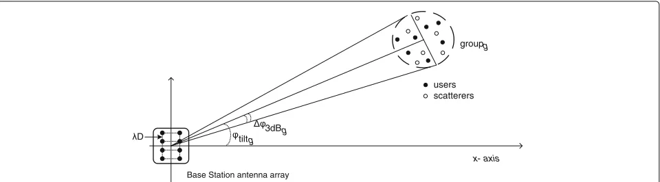
for 0≤i, j≤M−1, that are the index of the antenna posi-tion in the array andλDis the minimum distance between two antenna elements at the BS. In addition, please note that our model differs from [8] as we consider a group cor-relation matrix, where UEs are not necessarily collocated,
whereas in [8] authors consider that each collocated UE have the same correlation matrix.
To recall, when using the geometrical one-ring model, we consider a 120o sector, obtained by using directional radiating elements, assuming that the sector is centered
around the x axis (α = 0 azimuth angle), and that no
energy is received for angles α ∈/ [−π/3,π/3]. Also, uniform linear array is supposed, so that the covariance
matrix Rg of the channel for a group g, with angle of
arrival (AoA)ϕtiltg and with angular spread of departure
ϕ3dBg= ϕ3dBg2 to groupg, can be used in (17).
Base Station antenna array
D 3dB
g
tilt
users scatterers
x- axis group
g g
The downlink channel of thegth group is expressed by applying the Karhunen-Loeve model, as
Hg=
diagonal matrix containing the non-zero eigenvalues of Rg, where Rg is of rank rg. Ug ∈ CM×rg is the
associ-ated eigenvectors matrix. The elements ofGg ∈ Crg×Kg
are distributed according toNC(0, 1). Also from (18), we
can observe that the knowledge ofRg is enough to
char-acterized Hg. This highlights the relationship between
the correlation matrix and the channel matrix for users belonging to groupg.
Then, as in [8,18], we use a two-tier precoder (TTP) scheme for FDD massive MIMO systems, and the trans-mitted signal is expressed as
x=
G
g=1
BgWgPgsg, (19)
whereBg ∈ CM×bgrepresents the outer precoder for the
groups, or Beamforming matrix while the inner pre-coder, or individual precoder isWg∈Cbg×Kgand depends
on the short-term effective channelH˜g = BHgHg. bg is
an integer design parameter,Pg ∈CKg×Kg is the diagonal
power allocation matrix√P/K×IwhereIis the identity matrix andsg ∈ CKg represents the data streams for the
gth group UEs.
Then, in comparison with the case where there was only one VSC (10) and (11), the received signal ygk and the
4.2 Codebook and feedback scheme
In FDD, the feedback problem is complex as the down-link and updown-link do not share the same band, hence, no reciprocity could be used. A classical way is to estimate the downlink channel from a training phase and then fed back to the BS via uplink signaling. This scheme could introduce feedback overhead in case of large amount of antenna at the BS as it is the case in massive MIMO where the downlink training represents a significant amount
of information. This feedback overhead will degrade the benefits of massive MIMO. Also a new feedback scheme has been introduced by Verizon where the BS periodi-cally transmits beams at different angles by transmitting beam reference signal, also known as beam sweeping. UE maintains a candidate beam set and report the one with best beam reference signal received power [25]. We could extend beam sweeping to group of UEs and then perform the VSC. Another way is to consider a predefined code-book that is available at the UE and at the BS. As we are working in FDD, and in order to reduce the feedback overhead, we will provide a grouping feedback scheme.
As it can be seen in (20), the outer precoderBg is in
charge of the grouping interference. This means that by effectively choosing this outer precoder, it can help can-celing the effects of grouping interference. Information on the grouping downlink channel is needed for good outer precoder selection. As expressed in (18), correlation matrixRgis enough to learn the downlink channel of the
gth group, andRgdepends on the angle information given
by the knowledge of the hotspots location. By knowing the gth hotspot center location, its radius and the BS location,
we can compute the correlation matrixRg and
accord-ingly choose the outer precoderBgin order to avoid group
interference.
Those previous inputs enable us to compute ϕtilt and
ϕ3dB= ϕ3dB2 corresponding to the detected hotspot. We consider the following predefined codebook:
C=(ϕtilt,ϕ3dB)i,i=1, 2,. . ., 2B
(22)
The values of the angles are compared with those in the codebook, where angles matching gives us the
corre-sponding indexi. While this index is known by the BS,
whether because it has been given by a specific UE belong-ing to the hotspot or because it has been computed by the BS itself, we can select the pre-computed correlation matrix corresponding to the couple angles given by index iand then the outer precoder. The BS is now aware of the best precoding intended for this group and will apply it in order to focus the directive beam on the detected hotspot. For the individual precoderWg, also called inner
pre-coder, we can apply the same procedure as in Section3
and consider only one hotspot or we can use the method-ology given by [26]. There the UEs benefit from D2D tech-nology and exchange their CSI such that a cluster head (CH) is aware of the global CSI and select the adequate precoder for each UE.
5 Group localization
To be able to implement the VSCs, we have to character-ize their center and their radius. In this section, we aim to develop algorithms to identify these two values depending on the operator strategy. Therefore, our algorithm is able to automatically detect hotspots and dynamically iden-tify a variation of these two characteristics allowing the network to adapt in real time its coverage.
5.1 UEs mapping using Global Positioning System Here we respond to the missing point of hotspot location by proposing a dynamic clustering algorithm based on Global Positioning System (GPS) coordinate location. We suppose that the BS benefits from minimization of drive tests (MDT) [27] which collects network quality informa-tion like UE coordinates, i.e., MDT geo-localize the UEs. Detailed location information provided by MDT reports, allows the operator to associate a set of MDT measure-ments with a physical location. The UEs are requested by the BS to acquire location information for a configured
MDT session [28]. The knowledge of the UEs coordinates
is hence available at the BS and can be used in order to find the hotspots. The BS will apply an algorithm based on the well known K-means that outputs or create clus-ters of UEs. Then, after some optimizations, we succeed on transforming the clusters into hotspots.
The general algorithm for hotspot detection is
con-structed as in [14]. First, K-means is an unsupervised
learning algorithm that solves clustering problem. In
K-means, a set of K data points and an integerC which
represents the number of centers to evaluate are given. These centers are randomly defined and then optimized in order to minimize the mean squared distance from each data point to its nearest center [29], as described between the lines 1 and 15 in Algorithm 1. Then, the optimal num-ber of clusters is selected based on the distortion function provided by [30], as explained in Algorithm 1 in lines 16 to 23. Secondly, to avoid UEs located far from the cluster and still grouped to it by K-means, a process that removes the far UEs is implemented, which is presented between lines 24 and 32. Also, please notice that if a cluster is considered as low populated it will be removed from the database,
wherenis a parameter configurable by the operator. The
last optimization is on determining if the cluster can be smaller covering almost the same number of UEs by look-ing each cluster density thanks to their distortion values. Parameterpline 37 represents a fraction of the inter site distance.
In order to evaluate the potential of our algorithm, let us consider a system composed of 57 hexagonal cell with inter site distance (ISD) of 500 m. Then, in each cell, we have “created” a circle of 40 m radius and randomly placed 60% of the UEs inside and 40% outside this circle, as rep-resented in Fig.4. We consider perfect GPS localization.
Algorithm 1Hotspot identification
BS requests for immediate MDT data from the subscriber UE Input:K,(xk,yk)k={1,...,K},Cmax=3 Determine nearest center for each UE fork=1 :Kdo
Estimate the distortion for each cluster: fori=1 :Cdo
Total distortions:SC= C
i=1
Ii
Determine estimation functionf(C)withd(dimension) andαC(weight factor)
f(C)=
Select the optimal number of clusters: Copt=arg minCi=1,...,Cmaxf(Ci), and letMCopt
Compute the average distortion of each cluster ¯IC = IC
|UC|
if¯IC>pthen
Recompute this algorithm from line 25
40: else
Compute cluster radiusrCopt(C)=rC
end if end for
The error GPS localization will be taken into account in
Section6. When applying the proposed hotspot
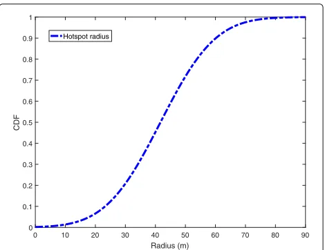
identifi-cation algorithm to each cell and by repeating the process 100 times, we obtain a probability of 55% of detecting one hotspot per sector, 41% of detecting two hotspots and 4% of detecting three hotspots. This means that new groups of UEs have been detected. Also, the hotspot identification algorithm is covering 72% of the total population which is 12% more than the considered cellular system. Further-more, after repeating the process hundred times, half of the radius measured are between 30 and 45 m, as it can be seen in Fig.8.
In Fig.9, 25% of the radius are below 32.7 m, half of the radius are below 39.4 m and 75% of the radius are below 50 m. A nearly Gaussian distribution for the cluster radius is observed which means that the closest value from the mean are more able to appear than the others. This is satisfactory as half of the clusters radius are close to 40 m. Now that the BS is aware of the center location and radius of the detected hotspot, the couple(ϕtilt,ϕ3dB)can
be computed thanks to (3) and (4), then a comparison
is made between this couple of angles and the ones in the predefined codebook C in (22). The index i,
corre-sponding to the closest couple in C with respect to the
calculated one, is chosen and gives the pre-computed
cor-relation matrix corresponding to index i and then the
outer precoder is deduce as explained in Section4.2. However, depending on the operator strategy, it might be more interesting to have a centralized hotspot localiza-tion at the UE side such that the BS is not overcharged by the UEs data. Furthermore, GPS provides a meter accuracy, which might be non-sufficient. In the next sub-section, UEs are localized based on radio links.
5 10 15 20 25 30 35 40 45 50 55 60 65 70 75 80 85 90
Fig. 8Clusters radius distribution. This histogram represents the results on an analysis on a hundred of iterations that have been performed and half of the radius measured are between 30 and 45 m
0 10 20 30 40 50 60 70 80 90
Fig. 9Statistics on hotspots radius. This figure represents a CDF of the hotspots radius where 25% of the radius are below 32.7 m, half of the radius are below 39.4 m and 75% of the radius are below 50 m. A nearly Gaussian distribution for the cluster radius is observed which means that the closest value from the mean are more able to appear than the others
5.2 UE mapping using direct radio links
In this section, instead of studying a centralized posi-tioning algorithm at the BS, as presented in the previous subsection, we will provide a UE level algorithm using only distances between the UEs. In that sense, we sup-pose that all the UEs are able to directly communicate between each other, i.e., they have D2D communication capability, where this technology has been added to the 3GPP release 12 [31]. Usually, studies on D2D are about increasing the data rate [32] or extending coverage. It has also been proved that within a certain distance it is bet-ter to communicate through D2D than passing through the cellular BS [33]. In this paper, we would like to cre-ate a map of all the UEs by exchanging information in order to detect neighbors devices as in [34–36]. The infor-mation exchanged will be only distance parameters and
no angles as in [34], as the axis of the mobile device
depends on current orientation or altitude which implies that the angles are perpetually changing. Before going further, we are going to see how can the distances be mea-sured between two devices without angle information and without anchor nodes, as in [35]. In order to detect the neighbor UE with highest possible accuracy, we propose to consider ultra-wideband (UWB) signals between the UE, which will help to provide D2D positioning. UWB is part of the IEEE 802.15 working group which specifies wireless personal area network (WPAN) standards [37]. In that sense, we may expect a future use of UWB for D2D communications.
against interference and fading, unlike ultrasound or infrared. Furthermore, UWB has low energy consumption [38] and very high accuracy thanks to its wide frequency
band [39] as it is indicated by Cramer–Rao lower band
(CRLB) [40]. A disadvantage of UWB is its coverage range which can be solved thanks to a well organized rout-ing topology between the smart devices, as explained
in Section 5.2.3. From the ranging techniques
perspec-tive, time of arrival (ToA) is a one-way time difference between the moment the receiver detects the transmit-ters’ signal and the time when the transmitter sends the signal. Usually, ToA offers a better accuracy than received signal strength and AoA for UWB positioning systems thanks to the high time resolution. Fortunately, due to the large bandwidth of UWB signal, multi-path compo-nents are often resolvable without the use of complex
algorithms [41]. And due to existing high performance
ToA estimation for UWB in NLOS [42–44], we will focus on this ranging technique. In order to work with ToA, we need to suppose perfect synchronization between the UEs.
Now that signal localization and ranging techniques are known, we will start the localization.
5.2.1 Group mapping methodology
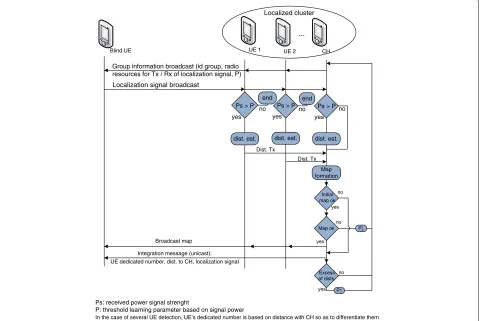
First of all, a CH is chosen according to the desired strat-egy, e.g., in [45] authors select for each VSC a CH that will be in charge of connecting all the UEs belonging to the same VSC. In our paper, a CH has a specific proces-sor capable of generating the treatment of the algorithm map, in order to represent the UEs in part of an area. The CH is also the first UE launching the algorithm procedure. As described in Fig.10, first the CH will broad-cast an information group message to the neighbors’ UEs including a group ID, radio resources for transmission and reception of localization signal and also a threshold
P of power limit. Once an unlocalized UE, called blind
UE, receives the information group message, if this UE is interested by joining the group, he will broadcast back a positive response to the UEs already localized by using the radio resources provided by the CH. Evaluated distance between the transmitter and the receiver will be transmit-ted to the CH. During the initialization step of the map, as we have a limited distance knowledge of the neighbor UEs, any blind UE is able to integrate our map as long as the threshold received powerPis satisfied. The initializa-tion map is the smallest possible map that we are able to
UE 1 UE 2 CH
Localized cluster
Ps > P Ps > P Ps > P yes yes yes
Map formation
Map ok
yes no
Ps: received power signal strenght
P: threshold learning parameter based on signal power
In the case of several UE detection, UE’s dedicated number is based on distance with CH so as to differentiate them
dist. est. dist. est. dist. est.
Dist. Tx
Dist. Tx Localization signal broadcast
Broadcast map
no no Group information broadcast (id group, radio
resources for Tx / Rx of localization signal, P)
no end end
Initial map ok
no
yes
Integration message (unicast): UE dedicated number, dist. to CH, localization signal
Excess of dists.
no
P yes
P
...
Blind UE
form, and is composed of at least four UEs as stated in the Proposition1and proved in a previous work [16].
Proposition 1With only n= 4UEs and the knowledge of Cn2 = 6distances named dij ∈ Rbetween UE i and
j (∀{i,j}ni=1,j>i), we can map the n UEs in an orthonormal coordinate system where the origin corresponds to the CH or any other UE.
CH is included within these four UEs. He is aware of the six distances between them, and each distance provides an equation such as
dij= (yj−yi)2+(xj−xi)2 (25)
between UEiandj, with four unknown values (each UE
has two coordinates). We then have six equations of this type for the case of four UEs (eight unknown values). Actually, as the wanted map is relative to the CH, we can consider that the CH coordinates are at the origin of the map and are (0, 0). So we finally have six equations for six unknown values, that consist of a solvable system of equations. Once the initial map is formed, this means that we have a map of at least four UEs. Then, when a blind
UE k wants to join the map, if an already localized UE
receives a signal from the previous one with a received powerPk < P, the algorithm will not be launched as we
consider only the reliable signals for distance estimation. Trilateration method is enough in order to add a blind
UEkto our map, as we need the distances between the
new UE and three other UEs (h,i, andj) already localized. The blind UEkis located at the intersection of the three circles of centerh, i, andj and radius dhk, dik, anddjk,
respectively. The three distances used to localize the blind
UE k correspond to the three most accurate distances
selected thanks to the received power. If the threshold
powerPis too high such that the CH does not collect at
least three signals,Pwill be reduced at the next iteration. Finally, if a UE is added to the map, a broadcast of the map is possible and an integration message is sent by the CH to the new UE.
Proposition 2With n > 4, a map can be created with only6+3(n−4)<Cn2distances.
Proposition2, provided in [16] means that we do not need to know all the distances between all the UEs in order to form a map. In order to add a blind UE to our map, we will need to solve a system of three equations such as (25). Also for good accuracy of the system, we will accept an incertitude of +/−xmeters in order to solve our system of equations. It will give output a location zone for blind UE called measurement incertitude, as represented in Fig.11,
d3
d2
Blind UE
d1
Fig. 11Measurement incertitude model. This figure represents a location zone for blind UE called measurement incertitude zone, where the white UE are the already localized ones and the red one represents the blind UE
where the white UEs are the already localized ones and the red one represents the blind UEk.
If the system of equations provides no solution, i.e., no location zone, this means that one of the distance values does not match with the others, which may happen in case of strong error estimation of a distance. If this occurs, the CH will look for another distance, called redun-dant distance, possibly available at the CH as detailed in Corollary1.
Corollary 1In the case of mapping failure due to error distance estimation (n > 4), we benefit from additional n−4redundant distances to create a map.
When adding UEninto a map, we benefit fromn−1 new possible distances. In order to add this new UE into the map, we only need additional [6+3(n−4)]−[6+3(n− 1−4)]=3 distances (i.e., based on Proposition2). So we benefit fromn−1−3=n−4 additional distances in case of mapping failure. The redundant distances are directly affected by the thresholdP, as higherPis, less redundant distances will be available. If no solution is provided by our system of equations, we reduceP. But even with such selection, the zone where blind UEkis possibly localized is still inaccurate.
5.2.2 Accuracy improvement
Algorithm 2 needs as input parameters the set of the three
best distancesDbetween the blind UE and the groupUof
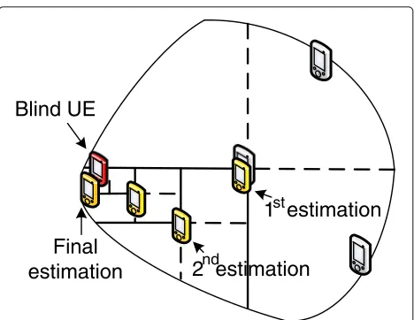
already localized UEs. The goal of the algorithm is to tight this zones, given by trilateration, by dividing it into sub zones and selecting the appropriated one. The procedure is based on dichotomy research where the value parame-ter for selection is represented by line 13 in Algorithm 2. Each iteration gives output a more accurate zone where its center is selected as the estimated location of the blind UE. All these steps are detailed in Algorithm 2, and once we apply this algorithm to the previous measurement incertitude zone (Fig.11), we see an improvement of the accuracy as our estimated position is closer to the real one (Fig.12).
Algorithm 2Map accuracy
Require: Estimated distancesD = {d1,d2,d3}between the new UE and the UEs already localizedU = {UEi= (xi,yi)|i∈[ 1,|D|]}
FromD, we get the estimated zoneZprovided by the measurement incertitude in the general map
compute center and perimeter ofZ:cZandPZresp.
3: Estimated UE:Est_ue=cZ
whilePZ> εdo
Divide the zone into four sub zones {z1,z2,z3,z4} where border meet atcZ
6: Compute their centers and perimetersC = {c1,c2,
c3,c4}and{P1,P2,P3,P4}resp. fori=1 :|C|do
Sumi=0
9: forj=1 :|D|do
d2j,ci=(yj−yci)2+(xj−xci)2
Sumi=Sumi+
d2j,c i−d
2 j
12: end for
end for
Z=zkandPZ=Pkwherek=arg mink∈[1,|C|]Sumk 15: Est_ue=cz
end while
5.2.3 UWB coverage extension and multi-group detection
As the coverage of UWB is limited to around 20 m [46],
this rang has to be increased in order to satisfy the VSCs coverage specifications which is around 40 m, as the VSCs are supposed to replace the picocells. One obvious option is by relaying the UWB signals. Let us now introduce UEs that have relaying capabilities. Our network is hence composed of four type of UEs:
• The CH, which is the one that launches the localization procedure and computes its corresponding map.
1 estimation
Blind UE
Final
estimation
2 estimation
st
nd
Fig. 12Blind UE positioning accuracy applying Algorithm 2. This figure represents a location zone for blind UE after the optimization provide by Algorithm 2, where the yellow UEs are the estimated localization at each steps. The red one represents the blind UE
• The localized UE, which has been detected by a group. Its position is known by the CH. Once a localized UE belongs to a group, it stops listening to others group information signals.
• The blind UE, which has not been localize by any group and is still listening to group information signals.
• The relaying UE, that is localized at the border of its corresponding groups and is still listening to group information signals. Its goal is to relay the broadcast localization signal send by the CH in order to extend the coverage. It is elected as relaying UE by any UE that is transmitting the group information broadcast signal, i.e., by a CH or any other relay.
We suppose that each UE is composed of a frame that is divided into three subframes, one for the group ID, one for the role of the UE (CH, relaying, localized, or blind UE), and one for the number of hops to the CH.
As mentioned in Section 5.2.1, the CH is computing
the localization map (see Fig. 10). Once the maximum
UWB coverage rang is achieved and the map is performed, the CH will select the relaying UEs localized in the bor-der of the group. All these UEs will be informed by the CH of their group ID, role (localized or relaying UE) and number of hops to the CH. Then, the relaying UEs will extend the UWB coverage by retransmitting the group information broadcast signal intended to the still blind UEs and repeat the same procedure until no UEs are localized.
In the case that a relay from groupg detects a CH or
be one hotspot instead of two. In such a case, relay from
groupgandhwill compare their corresponding hops
sub-frame, and the one with less number of hops with its corresponding CH will change of group. Automatically, all the UEs attached to the relay that just made a group change will belong to the new group too. Their group ID subframe will change and the number of hops will be incremented. This is represented in Fig.13, whereUEgi
andUEhjare two relays belonging to two different groups
gandh, respectively. One of these relays detect the other, and they compare their subframe corresponding to the number of hops to their respective CH. Here, the num-ber of hops ofUEgiis 2 and the one ofUEhjis 1 so group
h will be integrated into groupg as represented in the
figure. Also, the number of hops in the subframe ofUEhj
is now 3 and the role ofCHh has changed into relaying
UE and its corresponding number of hops is now 4. Now that the coverage extension of UWB localization is no more a problem, we can apply part of the Algorithm 1 in order to transform the map of a group of UEs into a map of hotspot.
5.2.4 Results for UE mapping using UWB signals
We will now apply our UWB localization method and see how accurate it is in line of sight (LOS) and NLOS outdoor environment.
The channel model used below respects the IEEE 802.15.4a standards for UWB. As we are following the
European regulation, we selected the best bandwidth B
which is 1 GHz centered infc = 3993.6 MHz wherefc
represents the carrier frequency [47]. We recall the
pathloss model defined in IEEE 802.15.4a standards for UWB:
PL=PL0+10nlog(d) (26)
where PL represent the pathloss, PL0(dB) andnare spe-cific values depending on the channel model.dis the real distance between the transmitter and the receiver [46]. The signal to noise ratio (SNR) is expressed as
SNRdB=Pt−PL−Pn (27)
where Pt and Pn are the transmitted and noisy power,
respectively. From the standards [46], their power density
are equal to−41 dBm/MHz and−174 dBm/Hz,
respec-tively. As our bandwidth isB = 1 GHz,Pt = −41 dB
andPn = −114 dB. Because we use estimated distances
as input, we focused on the CRLB distance error which is one of the most commonly used measure of ToA accu-racy [40]. From [41], the accuracy of ToA can be improved by increasing the SNR or the effective signal bandwidth. Since UWB signals have very large bandwidths, we ben-efit from extremely accurate location estimation using ToA via UWB radios. Also an approximation method of
the CRLB when using UWB signals is introduced in [48]
and an other one using millimeter-wave (mm-wave) is proposed in [49]. The distance error,dCRLB, is given by the CRLB and the estimated distance isd+dCRLB, where
dCRLB≈
c 2πB√SNRWatt
(28)
The measurements were done following the IEEE
802.15.4a standards for LOS and NLOS in outdoors [46].
CH
Relay user Localized user
UE
hj gi
h g
CH
CH
CH h
CH
UE
UE
UEhj g
gi
Figure14presents the repartition depending on the error between the blind UE position and the estimated position for LOS and NLOS outdoor. These results are obtained after 100 simulations. The simulation results show that the localization accuracy in LOS environments has an estima-tion error below 2 cm in 73% of the cases and below 55 cm in 71% of the case in NLOS environments. Please notice that half of errors estimation are below 1 cm in LOS. Also, for LOS static UEs, [50] considered the performance of minimum mean squared error (MMSE) localization, where the difference between the true position and the
MMSE estimate position is presented in their Fig. 14.
Major part of their estimations are around 3 cm accuracy. In the next section, we compare our results to GPS approach used in our first group localization method in
Section 5.1 whose error localization will be considered
and is around 10 m in LOS outdoor environment [51];
as GPS remains the notorious outdoor localization tech-nique. Meanwhile, we propose a solution for the step after ToA estimations, several works focus on resolving the
most common problems of ToA signals [52–55]. Please
notice that we can achieve even better results with our
algorithm while combining these two visions, i.e., use effi-cient ToA as input to our algorithm. The CHs have now the maps of the hotspots from its point of view, i.e., from the orthonormal coordinate system where it is located at the origin.
Remark 1When creating such a map, we observe infi-nite solutions depending on the orthonormal coordinate system, but all the solutions will provide the same map with some rotation between 0 and2π. Uniqueness of the map can be achieved by fixing the coordinate system, i.e., by the knowledge of the cellular coordinate of one UE (different than the CH).
So, supposing that the CH is aware of its cellular coor-dinates and also the ones of another UE in its map, it will be able to compute the center location and radius of the mapped hotspot. The couple(ϕtilt,ϕ3dB)are deduce
from (3) and (4), then a comparison is made between this couple and the ones in the predefined codebookCin (22),
available at CH side. The indexi, corresponding to the
closest couple inCwith respect to the calculated one, is chosen and fed back to the BS. As only the CH is feeding back to the BS and not all the UEs, this will avoid feed-back overhead for the case of large amount of transmit
antennas. The BS can now choose the pre-computed
cor-relation matrix corresponding to index i and then the
outer precoder is deduced and applied in order to focus the directive beams on the detected hotspots.
6 Results and discussion
As our hotspot localization methods are intended for the use of the VSCs, we consider a cellular system with 150 UEs distributed in such a way that in each sector 60% of the UEs are clustered in a 40 m hotspot radius and the rest are randomly distributed (i.e., like if there was a picocell in a cellular sector). We apply our two hotspot localiza-tion methods for 100 simulalocaliza-tions and have highlighted four representative clustering realizations depending on UEs distribution, as shown in Fig.15. In realizationi, pre-sented in Fig.15a, both methods give us a hotspot where the one given by UWB signals has a smaller radius than the one given by the GPS, in particular, due to the GPS error localization of 10 m in average [51]. Figure 15b highlight a second representative realization where the 40% of the UEs, that are outside the predefined hotspot, are distributed in such a way that they form a second hotspot in the cellular sector. Meanwhile, both clustering methods detect this hotspot, its radius is much smaller using UWB method than GPS and also seems to be more
dense. Figure15c,dillustrate a quite similar repartition as in both cases the 60% of the UEs forming the predefined hotspot of 40 m radius can actually be separated into two sub-hotspots. By using GPS for hotspot detection, within these two cases, only the predefined hotspot is detected by the method whereas UWB detects the two sub-hotspots. In realizationiv, UEs close to the predefined hotspot are taken into account by the UWB method, and are included
into the final detection. Figure16represents the
cumu-lative distribution function (CDF) of the UE density per square meter for the detected hotspots with both meth-ods and we observe that UWB provide much more dense hotspots than GPS method. Also, it is important to note that the hotspots radius are in general smaller using UWB than using GPS as it can be seen in Fig.17, where the CDF of the hotspots radius is represented for both methods. Generalizing, as more precise the localization system is, the better the clustering results would be. Nevertheless, when selecting localization method, other criteria should also be taken into account such as the complexity, bat-tery consumption, terminal cost, etc. As our objective is to implement VSCs based on hotspot localization, it is important to focus the beamforming signal on a dense and accurate hotspot such that the energy and the resources used while performing the VSCs are optimal.
7 Conclusions
This work presents and proposes the concept of VSC as an alternative to classical heterogeneous networks (HetNets) deployed in 4G. Nowadays, the deployment of small cells in 4G implies a non-negligible cost in terms of new equip-ment deployequip-ment, sites acquisition, and maintenance for operators. In future wireless networks, the use of large
0 0.01 0.018 [...] 0,4 0,5 0,6 0,7 0,8 0,9
Fig. 16CDF of the UE density perm2depending on the localization method. This figure represents the CDF of the UE density per square meter for the detected hotspots with both methods and we observe that UWB provide much more dense hotspots than GPS method
0 10 20 30 40 50 60 70 80 90
Fig. 17CDF of the hotspots radius depending on the localization method. This figure represents the CDF of the radius where the hotspots radius are in general smaller using UWB than using GPS
terms of coverage and avoiding architecture constraints. Once the hotspots have been successfully localized, a new codebook has been defined based on hotspot information, consequently reducing the feedback to the BS and pro-vides suitable precoding in order to improve the accuracy of the highly directive beams.
Abbreviations
3GPP: 3rd Generation Partnership Project; BS: Base station; D2D: Device-to-device; GPS: Global Positioning System; LOS: Line of sight; MDT: Minimization of drive tests; MIMO: multiple input multiple output; NLOS: Non-line of sight; ToA: Time of arrival; UE: User equipment; UWB: Ultra-wideband; VSC: Virtual small cell
Acknowledgements
The authors would like to thank Siham Arreffag for her help in the second positioning method.
Funding
The work is supported by Radio link Innovative DEsign (RIDE) team belonging to Orange Labs Networks, France
Authors’ contributions
TVS made the main contribution on system modeling, codebook design and on methods for positioning. While SML helps out with the second positioning method, AGS supervise the first one. The concept of VSC has been originally propose by both of the co-authors AGS and SML. Finally all authors read and approved the final manuscript.
Competing interests
The authors declare that they have no competing interests.
Publisher’s Note
Springer Nature remains neutral with regard to jurisdictional claims in published maps and institutional affiliations.
Received: 1 November 2017 Accepted: 4 June 2018
References
1. H Holma, A Toskala, J Reunanen,LTE small cell optimization: 3GPP Evolution to Release 13. (John Wiley & Sons, United Kingdom, 2016)
2. J Hoydis, M Kobayashi, M Debbah, Green small-cell networks. IEEE Veh. Technol. Mag.6(1), 37–43 (2011)
3. A Osseiran, F Boccardi, V Braun, K Kusume, P Marsch, M Maternia, O Queseth, M Schellmann, H Schotten, H Taoka,et al, Scenarios for 5G mobile and wireless communications: the vision of the METIS Pproject. IEEE Commun. Mag.52(5), 26–35 (2014)
4. S Katikala, GoogleTMProject Loon. InSight: Rivier Acad. J.10(2), 1–6 (2014) 5. F Rusek, D Persson, BK Lau, EG Larsson, TL Marzetta, O Edfors, F Tufvesson,
Scaling up MIMO: opportunities and challenges with very large arrays. IEEE Signal Proc. Mag.30(1), 40–60 (2013)
6. S Shalmashi, E Björnson, M Kountouris, KW Sung, M Debbah, Energy efficiency and sum rate tradeoffs for massive MIMO systems with underlaid device-to-device communications. EURASIP J. Wirel. Commun. Netw.2016(1), 175 (2016)
7. C Shepard, H Yu, N Anand, E Li, T Marzetta, R Yang, L Zhong, in Proceedings of the 18th Annual International Conference on Mobile Computing and Networking. Argos: practical many-antenna base stations (ACM, Istanbul, 2012), pp. 53–64
8. A Adhikary, J Nam, J-Y Ahn, G Caire, Joint spatial division and
multiplexing—the large-scale array regime. IEEE Trans. Inf. Theory.59(10), 6441–6463 (2013)
9. A Galindo-Serrano, SM Lopez, A De Ronzi, A Gati, inVehicular Technology Conference (VTC Spring), 2015 IEEE 81st. Virtual Small Cells Using Large Antenna Arrays as an Alternative to Classical HetNets (IEEE, Glasgow, 2015), pp. 1–6
10. Y Liu, X Duan, G Boudreau, A Bin Sediq, X Wang, inIEEE Global Communications Conference (GLOBECOM). Adaptive beamforming based
inband fronthaul for cost-effective virtual small cell in 5G networks (IEEE, Singapore, 2017)
11. VG Vassilakis, H Mouratidis, E Panaousis, ID Moscholios, MD Logothetis, in 24th IEEE International Conference on Telecommunications (ICT). Security requirements modelling for virtualized 5G small cell networks (IEEE, Limassol, 2017), pp. 1–5
12. A Radwan, MF Domingues, J Rodriguez, inIEEE International Conference on Communications Workshops (ICC Workshops). Mobile caching-enabled small-cells for delay-tolerant e-Health apps (IEEE, Paris, 2017), pp. 103–108 13. Q Zhang, J Zeng, X Su, L Rong, X Xu, inInternational Conference on
Communicatins and Networking in China. Virtual small cell selection schemes based on sum rate analysis in ultra-dense network (Springer, Chongqing, 2016), pp. 78–87
14. T Varela Santana, A Galindo-Serrano, B Sayrac, S Martínez López, inIEEE International Symposium on Wireless Communication Systems (ISWCS). Dynamic network configuration: hotspot identification for virtual small cells (IEEE, Poznan, 2016), pp. 49–53
15. A Dammann, R Raulefs, S Zhang, inIEEE International Conference on Communication Workshop (ICCW). On prospects of positioning in 5G (IEEE, Shah Alam, 2015), pp. 1207–1213
16. T Varela Santana, S Arreffag, S Martínez López, inIEEE International Symposium on Personal, Indoor and Mobile Radio Communications (PIMRC). A high resolution method for equipment group mapping using UWB signals (IEEE, Montreal, 2017)
17. H Li, L Han, R Duan, GM Garner, Analysis of the synchronization requirements of 5G and corresponding solutions. IEEE Commun Stand. 1(1), 52–58 (2017)
18. M Dai, B Clerckx, D Gesbert, G Caire, A rate splitting strategy for massive MIMO with imperfect CSIT. IEEE Trans. Wirel. Commun.15(7), 4611–4624 (2016)
19. X Rao, VK Lau, Distributed compressive CSIT estimation and feedback for FDD multi-user massive MIMO systems. IEEE Trans. Signal Process.62(12), 3261–3271 (2014)
20. R Di Taranto, S Muppirisetty, R Raulefs, D Slock, T Svensson, H Wymeersch, Location-aware communications for 5G networks: how location information can improve scalability, latency, and robustness of 5G. IEEE Signal Proc. Mag.31(6), 102–112 (2014)
21. S Fortes, A Aguilar-García, R Barco, FB Barba, JA Fernández-Luque, A Fernández-Durán, Management architecture for location-aware self-organizing LTE/LTE-a small cell networks. IEEE Commun. Mag.53(1), 294–302 (2015)
22. 3GPP TR 36.814 Evolved Universal Terrestrial Radio Access: further advancements for E-UTRA physical layer aspects (release 9). Technical report, 3GPP organization (2010)
23. D Maaz, A Galindo-Serrano, SE EL Ayoubi, inIEEE International Conference on Telecommunication (ICT) Workshop on Main Trends on 5G and Beyond Networks (MT5Gnet). URLLC User Plane Latency Performance in New Radio (IEEE, Saint Malo, 2018)
24. A Gati, S Martinez-Lopez, T En-Najjary, inWireless Communications and Networking Conference Workshops (WCNCW). Impact of traffic growth on energy consumption of LTE networks between 2010 and 2020 (IEEE, Istanbul, 2014), pp. 150–154
25. Testing 5G: Data throughput.https://literature.cdn.keysight.com/litweb/ pdf/5992-2519EN.pdf?id=2920715
26. H Yin, L Cottatellucci, D Gesbert, inIEEE 48th Asilomar Conference on Signals, Systems and Computers. Enabling massive MIMO systems in the FDD mode thanks to D2D communications (IEEE, Pacific Grove, pp. 656–660
27. 3GPP TS 37.320 V11.1.0 Universal Terrestrial Radio Access (UTRA) and Evolved Universal Terrestrial Radio Access (E-UTRA); radio measurement collection for minimization of drive tests (MDT); overall description; stage 2 (Release 11). Technical report, 3GPP organization (2012)
28. J Johansson, WA Hapsari, S Kelley, G Bodog, Minimization of drive tests in 3gpp release 11. IEEE Commun. Mag.50(11), 36–43 (2012)
29. A Likas, N Vlassis, JJ Verbeek, The global K-means clustering algorithm. Pattern Recognit.36(2), 451–461 (2003)
30. DT Pham, SS Dimov, CD Nguyen, Selection of K in K-means clustering. Proc IME C J Mech Eng Sci.219(1), 103–119 (2005)
32. T Varela Santana, R Combes, M Kobayashi, inIEEE International Symposium on Information Theory (ISIT). Device-to-Device Aided Multicasting IEEE, Vail, Colorado, 2018). June 17-22, 2018
33. R Ibrahim, M Assaad, B Sayrac, A Ephremides, inIEEE International Symposium on Wireless Communication Systems (ISWCS). Overlay D2D vs. cellular communications: a stability region analysis (IEEE, Bologna, 2017) 34. J-W Qiu, CC Lo, C-K Lin, Y-C Tseng, inIEEE Wireless Communications and
Networking Conference (WCNC). A D2D relative positioning system on smart devices (IEEE, Istanbul, 2014), pp. 2168–2172
35. N Patwari, JN Ash, S Kyperountas, AO Hero, RL Moses, NS Correal, Locating the nodes: cooperative localization in wireless sensor networks. IEEE Signal Proc. Mag.22(4), 54–69 (2005)
36. C Savarese, JM Rabaey, J Beutel, inIEEE International Conference on Acoustics, Speech, and Signal Processing, 2001. Proceedings. (ICASSP’01).vol. 4. Location in distributed ad-hoc wireless sensor networks (IEEE, Salt Lake City, UT, 2001), pp. 2037–2040
37. E Karapistoli, F-N Pavlidou, I Gragopoulos, I Tsetsinas, An overview of the IEEE 802.15. 4a standard. IEEE Commun. Mag.48(1), 47–53 (2010) 38. J Zhang, PV Orlik, Z Sahinoglu, AF Molisch, P Kinney, UWB Systems for
wireless sensor networks. Proc. IEEE.97(2), 313–331 (2009) 39. K Witrisal, S Hinteregger, J Kulmer, E Leitinger, P Meissner, inIEEE
International Conference on RFID. High-accuracy positioning for indoor applications: RFID, UWB, 5G, and beyond (IEEE, Orlando, Florida, 2016), pp. 1–7
40. WC Chung, D Ha, inIEEE Conference on Ultra Wideband Systems and Technologies. An accurate ultra wideband (UWB) ranging for precision asset location (IEEE, Reston, Virginia, 2003), pp. 389–393
41. S Gezici, Z Tian, GB Giannakis, H Kobayashi, AF Molisch, HV Poor, Z Sahinoglu, Localization via ultra-wideband radios: a look at positioning aspects for future sensor networks. IEEE Signal Proc. Mag.22(4), 70–84 (2005)
42. S Al-Jazzar, J Caffery, inIEEE 56th Vehicular Technology Conference. Proceedings. VTC 2002-Fall,vol. 2. ML and Bayesian TOA location estimators for NLOS environments, (2002), pp. 1178–1181
43. S Al-Jazzar, J Caffery, H-R You,A scattering model based approach to NLOS mitigation in TOA location systems, (2002), pp. 861–865
44. B Denis, J Keignart, N Daniele, inUltra Wideband Systems and Technologies, 2003 IEEE Conference On. Impact of NLOS propagation upon ranging precision in UWB systems (IEEE, Reston, Virginia, 2003), pp. 379–383 45. A Behnad, X Wang, Virtual small cells formation in 5G networks. IEEE
Commun. Lett.21(3), 616–619 (2017)
46. AF Molisch, K Balakrishnan, C-C Chong, S Emami, A Fort, J Karedal, J Kunisch, H Schantz, U Schuster, K Siwiak, IEEE 802.15. 4a Channel Model-Final Report. IEEE P802.15(04), 0662 (2004)
47. AF Molisch, P Orlik, Z Sahinoglu, J Zhang, inFirst International Conference on Communications and Networking in China. ChinaCom’06. UWB-based sensor networks and the IEEE 802.15. 4a Standard-a tutorial (IEEE, Beijing, 2006), pp. 1–6
48. J Zhang, RA Kennedy, TD Abhayapala, Cramér-Rao lower bounds for the synchronization of UWB signals. EURASIP J. Appl. Signal Process.2005, 426–438 (2005)
49. A Shahmansoori, GE Garcia, G Destino, G Seco-Granados, H Wymeersch, Position and orientation estimation through millimeter wave MIMO in 5G systems. IEEE Trans. Wirel. Commun.17, 1822–1835 (2017)
50. H Wymeersch, J Lien, MZ Win, Cooperative localization in wireless networks. Proc. IEEE.97(2), 427–450 (2009)
51. PA Zandbergen, Accuracy of iPhone locations: a comparison of assisted GPS, WiFi and Cellular Positioning. Trans. GIS.13(s1), 5–25 (2009) 52. G Fischer, O Klymenko, D Martynenko, H Luediger, inInternational
Conference on Indoor Positioning and Indoor Navigation (IPIN). An Impulse Radio UWB Transceiver with High-Precision TOA Measurement Unit (IEEE, Zurich, 2010), pp. 1–8
53. R Merz, F Chastellain, A Blatter, C Botteron, P-A Farine, inEuropean Navigation Conference, Toulouse, France. An experimental platform for an indoor location and tracking system (IEEE, Toulouse, 2008)
54. G Cheng, Accurate TOA-Based UWB Localization system in coal mine based on WSN. Phys. Procedia.24, 534–540 (2012)

![Fig. 5 SINR CDF at dense urban scenario [9]. This figure represents theSINRs of three scenarios, i.e., only macrocell, macrocell-VSC, andmacrocell-picocell scenarios](https://thumb-us.123doks.com/thumbv2/123dok_us/881351.1105898/7.595.57.541.86.291/scenario-represents-thesinrs-scenarios-macrocell-macrocell-andmacrocell-scenarios.webp)