Flow characteristics of 3 D turning diffuser using particle image velocimetry

Flow Characteristics of 3-D Turning

Diffuser using Particle Image Velocimetry

Normayati Nordin #1, Zainal Ambri Abdul Karim *2, Safiah Othman #3,

Vijay R. Raghavan **4, Mohd Faizal Mohideen Batcha #5, Azian Hariri #6, Siti Mariam Basharie #7

#

Flow Analysis, Simulation and Turbulence Research Group, Center for Energy and Industrial Environmental Studies, Faculty of Mechanical and Manufacturing Engineering, Universiti Tun Hussein Onn Malaysia

86400 Batu Pahat, Johor, Malaysia

1

[email protected]

*

Department of Mechanical and Manufacturing Engineering, Universiti Teknologi Petronas 31750 Tronoh, Perak, Malaysia

2

[email protected]

**

OYL Research and Development Center 47000 Sungai Buloh, Selangor, Malaysia

4

[email protected]

Abstract—It is often necessary in fluid flow systems to simultaneously decelerate and turn the flow. This can be achieved by employing turning diffusers in the fluid flow systems. The flow through a turning diffuser is complex, apparently due to the expansion and inflexion introduced along the direction of flow. The flow characteristics of 3-D turning diffuser by means of varying inflow Reynolds number are presently investigated. The flow characteristics within the outlet cross-section and longitudinal section were examined respectively by the 3-D stereoscopic PIV and 2-D PIV. The flow uniformity is affected with the increase of inflow Reynolds number due to the dispersion of the core flow throughout the outlet cross-section. It becomes even worse with the presence of secondary flow, 22% to 27% of the mean outlet velocity. The flow separation takes place within the inner wall region at the point very close to the outlet edge and the secondary flow vortex occurs dominantly within half part of the outlet cross-section.

Keyword- Turning diffuser, Flow Characteristics, Particle Image Velocimetry (PIV)

I. INTRODUCTION

It is often necessary in fluid flow systems to simultaneously decelerate and turn the flow. This can be achieved by employing turning diffusers in the fluid flow systems. A turning diffuser is characterised by its expansion directions into two types, namely, two dimensional (2-D) turning diffuser and three-dimensional (3-D) turning diffuser [1, 2, 3]. A geometric layout of a 90o turning diffuser is shown in Fig. 1. A 2-D turning diffuser expands its cross-section in either x-y or y-z axis plane, whereas a 3-D turning diffuser expands its cross-section in both x-y and y-z planes.

Chong et al. [4] designed a 90o turning diffuser with quadrants of circles at both the inner wall and centreline. The outer wall was shaped using circular arcs with the centres placed along the centreline and the circumferences tangent to the inner wall. It was designed such that equal area distributions were established between the inner and outer wall passages relative to the centreline. The gross geometry of a turning diffuser could be described in terms of four parameters, namely, the inner wall length to the inlet throat width ratio (Lin/W1), the outlet area to the inlet area ratio (AR) , the outlet-inlet configurations (W2/W1, X2/X1) and the turning

angle () [5].

The flow through a 90o turning diffuser is complex, apparently due to the expansion and sharp inflexion introduced along the direction of flow. The inner wall is subjected to curvature-induced effects where under a strong adverse pressure gradient, the boundary layer on the inner wall is likely to separate, and the core flow tends to deflect toward the outer wall region [2, 6]. Flow separation is basically undesirable as it would decrease the core flow area, induce the presence of secondary flow vortices and ultimately affect the flow uniformity [4]. The flow uniformity index (out) is used to measure the extent of dispersion of local outlet velocity from the

mean outlet velocity. The out was strongly dependent on the dispersion of core flow, y and the presence of

secondary flow, Sout throughout the outlet cross-section [7].

In the present work, the flow characteristics of 3-D turning diffuser of = 90o, AR= 2.16, W2/W1=1.440,

X2/X1=1.500 and Lin/W1= 3.970 are experimentally investigated. The operating condition is varied within the

Fig. 1. A geometric layout of a 90o _{turning diffuser}

II. INSTRUMENTATIONANDMEASUREMENTSETUP

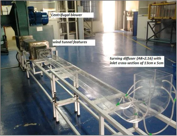
The test rig shown in Fig. 2 was developed. A centrifugal blower controlled using a 3-phase inverter and calibrated previously by [8] was installed at the upstream end. The rig was incorporated with several wind tunnel features to produce a fully developed flow at the diffuser entrance [9]. The test section, with inlet cross-section of 13 cm x 5 cm and hydrodynamic entrance length of 28Dh featured no fittings.

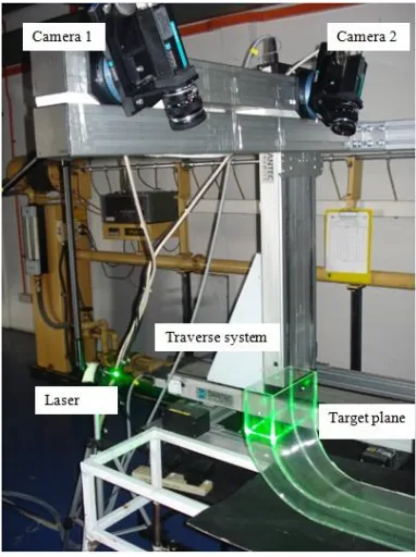
The outlet flow uniformity was examined using a 3-D stereoscopic PIV shown in Fig. 3. The measurement procedures are as follows:

1. Two CCD cameras were mounted on top of the target plane while their distance and angle (30o) were adjusted until both cameras could capture the target plane entirely.

2. The laser was calibrated to provide a perfect illumination and aligned to the target plane for marking. 3. Calibration for 3-D stereoscopic PIV was performed as follows:

a. The standard calibration target board of 200 mm x 200 mm was aligned to be parallel to the marked target plane, i.e. the first position.

b. The cameras were traversed to the calibration target. The zoom and aperture of each camera were adjusted optimally.

c. The CCD plane of each camera was tilted to satisfy the Scheimpflug condition, to provide best possible focus over the entire image.

d. The cameras were run in single frame mode and satisfactory calibration images were acquired and saved for calibration.

e. The target board was re-positioned by inclining 10 each its side at a time, i.e. the other four positions.

Fig. 3. 3-D stereoscopic PIV setup

Fig. 4. 2-D PIV setup

f. Steps 3 (d) and (e) were repeated until all the positions completed.

g. The recorded calibration images were selected and Image model fit (IMF)-Pinhole was adopted. h. A successful calibration was verified by superimposing the calibration IMF plots to the

corresponding calibration images. The accurate calibrations should provide the average reprojection error of less than 1.

i. The calibrated cameras were traversed back to the target plane.

4. The blower was turned on with the speed regulated to 9 RPM. Seeding particles were injected into the system. Measurements were made after 5 minutes to allow complete mixing between the air and the seeding particles.

5. The laser sheet was illuminated at the target plane with the thickness of 20 mm and the intensity of 10. The target plane was placed exactly at the center of the laser sheet.

6. The cameras were run in double frame mode. The time between pulses was set at 20µs. 100 images per camera were acquired and saved.

7. The images were divided into interrogation areas of 128 x 128 pixels. The 2-D velocity vectors, i.e. Vx

and Vz velocity components were calculated using cross-correlation.

8. The 2-D velocity vectors were filtered and subsequently masked to remove the unreasonable vectors. 9. The IMF calibration plots and the best 40 treated 2-D vector plots from both cameras were selected.

The 3-D velocity vectors, i.e. Vx, Vy and Vz were computed using stereo PIV processing. The 3-D vector

plots were selected and the local outlet velocity, Vi and mean oulet velocity, Vout were then calculated

using vector statistics.

10. The results were numerically and graphically extracted.

11. For verification, the third velocity component, Vy obtained by PIV was picked randomly at one point

and compared with the Pitot static probe result.

12. Procedure 6-11 was repeated by varying the time between pulses at 30µs, 50µs, 70µs, 90µs and 110 µs. The most optimum time between pulses should provide the least deviation between the PIV and Pitot static probe results. The confidence interval of the measured data to the repeatability of the experiments is within ±3.9% [10].

13. Procedure 4-13 was repeated by varying the blower speeds from 10, 15, 20 to 25 RPM. 14. The blower was turned off.

A 2-D PIV setup as shown in Fig. 4 was used to examine the flow characteristic at the centre plane within the longitudinal section. The measurement procedures are as follow:

1. The camera was arranged to be perpendicular to the target plane and its distance from the target plane was so adjusted that the target plane could be entirely captured.

a. The standard calibration target board 200 mm x 200 mm was aligned to be parallel to the marked target plane, i.e. the centre target plane.

b. The camera was traversed to the calibration target. The zoom and aperture of the camera were adjusted optimally.

c. The camera was run in single frame mode and a satisfactory calibration image was acquired and saved for calibration.

d. The recorded calibration image was selected and Image model fit (IMF)-DLT was adopted. e. A successful calibration was verified by superimposing the calibration IMF plot to the

corresponding calibration image. The accurate calibration should provide the average reprojection error of less than 1.

f. The calibrated camera was traversed back to the target plane.

4. The blower was turned on with the speed regulated to 9 RPM. Seeding particles were injected into the system. Measurements were made after 5 minutes to allow complete mixing between the air and the seeding particles.

5. The laser sheet was illuminated exactly at the target plane with the thickness of 2 mm and the intensity of 10.

6. The camera was run in double frame mode. 100 images were acquired and saved.

7. The images were divided into interrogation areas of 64 x 64 pixels. The velocity vectors within the turning diffuser were calculated using cross-correlation.

8. The velocity vectors were filtered and subsequently masked to remove the unreasonable vectors. The best 40 treated velocity vector plots were selected.

9. The results were numerically and graphically extracted.

10. Steps 4-9 were repeated by varying the blower speeds of 10, 15, 20 and 25 RPM. 11. The blower was turned off.

The flow uniformity index (out) was evaluated by calculating the mean standard deviation of outlet velocity.

The least absolute deviation corresponds to the greatest uniformity of flow [12]: 2 1 ) ( 1 1



out V V

N

 (1)

where,

N = number of measurement points

Vi = local outlet air velocity (m/s)

Vout = mean outlet air velocity (m/s)

The dispersion of core flow (y) was evaluated by calculating the standard deviation of axial velocity at the

outlet [11]: 2 1 ) ( 1 1



y V V

N

 (2)

where,

Vy = velocity in y-direction (m/s)

Vy avg = average velocity in y-direction (m/s)

Secondary flow index (Sout) represents the percentage of secondary flow at the outlet. The outlet velocity is

considered uniform only if secondary flow magnitude at the outlet is less than 10% of the mean outlet velocity [7]: out N i z x out V N V V S         

_

Vx = velocity in x-direction (m/s)

Vz = velocity in z-direction (m/s)

III. RESULTSANALYSISANDDISCUSSION

(a)

(b)

(c) Inner wall

Outer wall

Outer wall

Inner wall

(d)

(e)

Fig. 5. Characteristic of the core flow, Vy (represented by color-coded) and the resultant of secondary flows, Vx and Vz (represented by arrows)

at the outlet by varying (a) Rein=5.786Ex 104 (b) 6.382 x 104 (c) 1.027 x 105 (d) 1.397 x 105 (e) 1.775 x 105

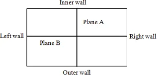
Velocity profiles are extracted across the centre of the turning diffuser outlet at two (2) different planes as shown in Fig. 6. As depicted in Fig. 7, the profiles are obtained to be asymmetric in each case. In Plane A, the flows deflect much toward the outer wall due to the existence of reverse core flows within the inner wall region. In Plane B, the secondary flow vortex occurs dominantly within half part of the outlet, i.e. left side causing the flow area in that particular region is to decrease.

Fig. 6. Velocity profile planes across the centre of turning diffuser outlet Outer wall

(a) (b)

Fig. 7. Velocity profiles at (a) Plane A and (b) Plane B

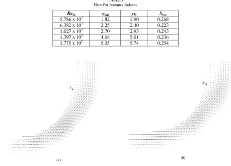
The out is affected with the increase of Rein as indicated in TABLE I mainly because of the dispersion of the

core flow, y throughout the outlet cross-section. It becomes even worse with the presences of the secondary

flow, Sout = 22% to 27% of the mean outlet velocity. The secondary flow vortices throughout the outlet

cross-section together with the excessive flow separation within the inner wall region may occur under a very strong pressure gradient and these not only incur unfavourable flow performance but also considerable losses associated with form drag [13, 14].

Vector plots, as in Fig. 8, demonstrate the flow structures within the longitudinal section of turning diffuser taken at the centre plane. Since the flow structures of each case are almost the same, in order to avoid repetition, only the flow structures of minimum and maximum Rein are included in the paper. The boundary layer in each

case separates from the inner wall almost at the same point which is close to the outlet edge, S= 0.9Lin/W1.

TABLE I Flow Performance Indexes

Rein out y Sout

5.786 x 104 1.82 1.90 0.268

6.382 x 104 2.25 2.40 0.223

1.027 x 105 2.70 2.93 0.243

1.397 x 105 4.64 5.01 0.236

1.775 x 105 5.05 5.74 0.254

(a) (b)

IV. CONCLUSION

In conclusion, the current work managed to investigate the flow characteristics of 3-D turning diffusers by means of varying Rein= 5.786 x 104 - 1.775 x 105. The flow uniformity is affected with the increase of Rein

mainly because of the dispersion of the core flow throughout the outlet cross-section. It becomes even worse with the presences of secondary flow, 22% to 27% of the mean outlet velocity. The secondary flow vortex occurs dominantly within half part of the outlet, i.e. left side causing the flow area in that particular region is to decrease. The flow separation takes place within the inner wall region close to the outlet edge of approximately 0.9Lin/W1. The non-uniformity of flow due to dispersion of core and secondary flows within the 3-D turning

diffusers shall be improved with baffles installment. This is for future work to undertake.

ACKNOWLEDGMENT

This work was financially supported by the Fundamental Research Grant Scheme (FRGS) of the Ministry of Higher Education, Malaysia and was conducted in Universiti Tun Hussein Onn Malaysia (UTHM). Immeasurable appreciation is extended to Head of Department of Energy and Thermofluid Engineering of UTHM, Assoc. Prof. Dr. Norzelawati Asmuin for all provided research supports. A sense of gratitude is extended to department members, especially Dr. Norasikin Mat Isa, Mr. Suzairin Md. Seri, Dr. Bambang Basuno and Dr. Hamidon Salleh for their insight sharing. Also thanks to Mr. Zainal Abidin Alias (Assistant Engineer of PIV Laboratory, UTHM) for the technical-lab assist.

REFERENCES

[1] G. Gan and S.B. Riffat, “Measurement and computational fluid dynamics prediction of diffuser pressure-loss coefficient,” Applied Energy, vol. 54(2), pp. 181-195, 1996.

[2] R.K. Sullerey, B. Chandra, and V. Muralidhar, "Performance comparison of straight and curved diffusers," J. of Def. Sci., vol. 33, pp. 195-203, 1983.

[3] N. Nordin, V.R. Raghavan, S. Othman and Z.A.A. Karim,“Compatibility of 3-Dturning diffusers by means of varying area ratios and outlet-inlet configurations", ARPN Journal of Engineering and Applied Sciences, Vol. 7, No. 6, pp 708-713, 2012.

[4] T.P. Chong, P.F. Joseph and P.O.A.L. Davies, “A parametric study of passive flow control for a short, high area ratio 90 deg curved diffuser,” J. Fluids Eng., vol. 130, 2008.

[5] C.J. Sagi and J.P. Johnson, “The design and performance of two-dimensional, Curved Diffusers,” J. Basic Eng. ASME, vol. 89, pp. 715-731, 1967.

[6] N. Nordin, V. R. Raghavan, S. Othman and Z. A. A. Karim, “Numerical investigation of turning diffuser performance by varying geometric and operating parameters”, Applied Mechanics and Materials, Vol. 229-231, pp. 2086-2093, 2012.

[7] M. K. Gopaliya, P. Goel, S. Prashar, and A. Dutt, "CFD Analysis of performance characteristics of S-shaped diffusers with combined horizontal and vertical offsets," Computer & fluids, vol. 40, pp. 280-290, 2011.

[8] N. Nordin, Z.A.A. Karim, S. OthmanandV.R. Raghavan, “Design & development of low subsonic wind tunnel for turning diffuser application”, Advanced Materials Research, Vol. 614-615, pp. 586-591, 2013.

[9]N.Nordin, Z.A.A. Karim, S.Othmanand V.R. Raghavan, “Verification of fully developed flow entering diffuser and particle image velocimetry procedures”, Applied Mechanics and Materials, Vol. 465-466, pp. 1352-1356, 2014.

[10] N. Nordin, S. Othman, V.R. Raghavan and Z.A.A. Karim, “Verification of 3-D stereoscopic PIV operation and procedures”,

International Journal Engineering and Technology IJET/IJENS, , Vol. 12, Issue 4, pp. 19-26, 2012.

[11] M.K. Gopaliya, M. Kumar, S. Kumar, and S. M. Gopaliya, "Analysis of performance characteristics of S-shaped diffuser with offset,"

Aerospace Science & Tech., vol. 11, pp. 130-135, 2007.

[12] W.A. El-Askary and M. Nasr, “Performance of a bend diffuser system: Experimental and numerical studies,” Computer & Fluids, vol. 38, pp.160-170, 2009.

[13] N.Nordin, Z,A.A. Karim, S.OthmanandV.R. Raghavan, The performance of turning diffusers at various inlet conditions, Applied Mechanics and Materials, Vol. 465-466, pp. 597-602, 2014.