Towards simplification of hydrologic modeling: identification of dominant processes

www.hydrol-earth-syst-sci.net/20/4655/2016/ doi:10.5194/hess-20-4655-2016

© Author(s) 2016. CC Attribution 3.0 License.

Towards simplification of hydrologic modeling:

identification of dominant processes

Steven L. Markstrom1, Lauren E. Hay1, and Martyn P. Clark2

1_{US Geological Survey, P.O. Box 25046, MS 412, Denver Federal Center, Denver, Colorado, 80225, USA} 2_{National Center for Atmospheric Research, P.O. Box 3000, Boulder, Colorado, 80307, USA}

Correspondence to:Steven L. Markstrom ([email protected])

Received: 23 November 2015 – Published in Hydrol. Earth Syst. Sci. Discuss.: 25 January 2016 Revised: 22 October 2016 – Accepted: 28 October 2016 – Published: 22 November 2016

Abstract. The Precipitation–Runoff Modeling Sys-tem (PRMS), a distributed-parameter hydrologic model, has been applied to the conterminous US (CONUS). Parameter sensitivity analysis was used to identify: (1) the sensitive input parameters and (2) particular model output variables that could be associated with the dominant hydrologic process(es). Sensitivity values of 35 PRMS calibration parameters were computed using the Fourier amplitude sensitivity test procedure on 110 000 independent hydrolog-ically based spatial modeling units covering the CONUS and then summarized to process (snowmelt, surface runoff, infiltration, soil moisture, evapotranspiration, interflow, baseflow, and runoff) and model performance statistic (mean, coefficient of variation, and autoregressive lag 1). Identified parameters and processes provide insight into model performance at the location of each unit and allow the modeler to identify the most dominant process on the basis of which processes are associated with the most sensitive parameters.

The results of this study indicate that: (1) the choice of per-formance statistic and output variables has a strong influence on parameter sensitivity, (2) the apparent model complexity to the modeler can be reduced by focusing on those processes that are associated with sensitive parameters and disregard-ing those that are not, (3) different processes require different numbers of parameters for simulation, and (4) some sensitive parameters influence only one hydrologic process, while oth-ers may influence many.

1 Introduction

It has long been recognized that distributed-parameter hy-drology models (DPHMs) are complex because of the sub-tlety and diversity of the hydrologic cycle which they aim to simulate (Freeze and Harlan, 1969; Amorocho and Hart, 1964). In this study, two different aspects of this complexity are addressed:

1. DPHMs have too many input parameters (Jakeman and Hornberger, 1993; Kirchner et al., 1996; Brun et al., 2001; Perrin et al., 2001; McDonnell et al., 2007). In this article, distributed parameters are defined as model inputs that remain constant through time, but can vary spatially across the landscape. Those who apply these models often have difficulty with understanding what these parameters are and how they are used in the model. Regularly, there are several parameters that may have similar effect on the computations or may con-strain the model in unintended ways (Hrachowitz et al., 2014). Despite the developer’s claims that these DPHMs are more or less physically based, often there are not measurements or data sources available for reli-able development of all of the input parameters. Duan et al. (2006) describes “a gap in our understanding of the links between model parameters and the land surface characteristics”. These unmeasured parameters, osten-sibly tangible, are really empirical coefficients when it comes to application and calibration (Samaniego et al., 2010).

Figure 1.Location map of the conterminous US showing the different geographic regions referred to this study.

Mayer and Butler, 1993; Ewan, 2011). Often, the mean-ing of output variables is not always intuitive and results sometimes can seem contradictory (e.g., when stream-flow does not seem to correlate with climate informa-tion). The result of these complex issues has led to the study of parameter interaction (Clark and Vrugt, 2006) and equifinality (Beven, 2006).

Developing effective DPHM applications require that the modeler address these two aspects of complexity at the same time (i.e., the uncertainty problem: “If I am uncertain when estimating input parameters, due to either incomplete or in-accurate information, what effect does it have on the out-put?”, and the calibration problem: “I know the output I want, which parameters should I change and how much should I change them?”) (Chaney et al., 2015; Reusser and Zehe, 2011). While the user of a DPHM can do nothing about the complexity of the model’s internal structure, the appar-ent complexity can be reduced by limiting the parameters and the affected output under consideration (as described by Jakeman and Hornberger, 1993; Hay et al., 2006).

Global parameter sensitivity analysis can determine the degree to which different values of parameters can affect the simulation of certain model outputs (Sanadhya et al., 2013). Furthermore, parameter sensitivity can be evaluated with re-spect to selected output variables, each representing a differ-ent aspect of the hydrologic cycle (hereafter referred to as processes). Sensitivity analysis of this form can be used to identify both the input parameters that are the most sensitive (i.e., the parameters that affect the simulation the most) and the dominant process(es) (i.e., those processes which are af-fected most, by the most sensitive parameters) according to the DPHM.

Any particular DPHM must necessarily be able to simu-late any and all hydrological processes that may occur any-where on the landscape. However, with the application of a DPHM to a specific site, it can become much less complex when the dominant hydrological process(es) are identified, as not all processes are active to the same degree. The

mod-eling problem becomes less complex to the modeler when hydrological processes not relevant to the modeled domain or watershed are removed from consideration (Wagener et al., 2003; Reusser et al., 2011; Guse et al., 2014; Bock et al., 2016). Related to this, various methods have been de-veloped that will group similar watersheds together for pur-poses of study (Wolock et al., 2004; Winter, 2001; Ali et al., 2012) or for parameter regionalization (He et al., 2011; Merz and Blöschl, 2004; Seibert, 1999; Vogel, 2005). In addi-tion, dominant process concepts have been explored by sev-eral researchers as a way to classify watersheds and natural hydrologic systems for the purpose of simplifying DPHMs (Sivakumar and Singh, 2012; Sivakumar et al., 2007). Some have suggested this approach for use as a possible classifica-tion framework (e.g., Woods, 2002; Sivakumar, 2004). Pfan-nerstill et al. (2015) developed a framework for identifica-tion and verificaidentifica-tion of hydrologic processes in simulaidentifica-tion models on the basis of temporal sensitivity analysis. Cuntz et al. (2015) describe a method of identifying only informative parameters as a screening step in order to reduce the effort required to perform global sensitivity analysis on the full pa-rameter space. McDonnell et al. (2007) discuss the possibil-ity of simplifying hydrologic modeling by identifying “fun-damental laws” so that over-parameterized models are not needed. However, in our opinion we have not made much progress on that front and DPHMs are, in many ways and for many reasons, more complex than ever.

(Chaney et al., 2015) and address the two aspects of com-plexity as described above.

2 Methods

2.1 Distributed-parameter hydrology model

The US Geological Survey’s Precipitation–Runoff Model-ing System (PRMS) is the DPHM used in this study. PRMS is a modular, deterministic, distributed-parameter, physical-process watershed model used to simulate and evaluate the effects of various combinations of precipitation, climate, and land use on watershed response. Each hydrologic process simulated by PRMS is encoded in a modular piece of source code (i.e., a “module”) and is represented by an algorithm that is based on a physical law (e.g., balance of energy re-quired to melt the ice in a snowpack) or empirical rela-tion with measured or estimated characteristics (e.g., a tank model used to simulate interflow). The reader is referred to Markstrom et al. (2015) for a complete description of PRMS. A fundamental assumption of this study is that PRMS is able to simulate and differentiate hydrologic signals from all the different processes at the scale of the CONUS. Two pos-sible ways to evaluate this are: (1) an analysis of PRMS’s internal structure, and (2) the history of PRMS applications. A detailed analysis of PRMS’s structure is beyond the scope of this article (see Markstrom et al., 2015); however, PRMS is implemented in a very linear fashion. Each parameter is clearly identified with an equation that is related to simu-lation of a specific process. Equations are solved sequen-tially, generally in the order that is defined by water moving through the hydrologic cycle, starting from the atmosphere as precipitation and moving through the rivers as streamflow. The outputs of one equation may be used as inputs to sub-sequent equations. All of the inputs for a particular equation are required before that equation can be solved. This inter-dependency in equations can lead to parameter interaction in the simulation of subsequent processes (as described by Beven, 1989; Grayson et al., 1992; Yilmaz et al., 2008; Pfan-nerstill et al., 2015). For example, parameters related to dis-tribution of temperature and solar radiation may show corre-lation with each other when evaluated with respect to sim-ulation of evapotranspiration, despite these parameters not being explicit terms in the evapotranspiration equations. Past studies indicate that PRMS has been very useful in water-resource and research studies across the CONUS (Battaglin et al., 2011; Boyle et al., 2006; Hay et al., 2011; Markstrom et al., 2012) and is capable of matching measured data (Bower, 1985; Cary, 1991; Dudley, 2008; Koczot et al., 2011) in a variety of geophysical and climatological settings.

To define the spatial domain for the CONUS application of PRMS, the locations of major river confluences, water bod-ies, and stream gages have been geo-referenced. Approxi-mately 56 000 stream segments are used to connect these

lo-cations. Using these stream segments, the left and right bank areas that contribute runoff directly to each segment have been identified, resulting in approximately 110 000 irregu-larly shaped hydrologic response units (HRUs) of various sizes (500 m2to 14 000 km2) (Viger and Bock, 2014). These HRUs are derived by their geographic and topographic loca-tion, affecting their extent and resolution. The CONUS appli-cation is forced with values of daily precipitation and daily maximum and minimum air temperature from the DAYMET data set (Thornton et al., 2014). The climate information cov-ers a time period from 1980 to 2013 on a daily time step, but a shorter period (1987–1989 used for warmup, and 1990–2000 used for evaluation) was used in this study.

2.2 Calibration parameters

The version of PRMS used in this study has 108 input param-eters. A parameter is defined as an input value that does not change over the course of a simulation run. Of these param-eters, most would never be modified from their initial val-ues (hereafter referred to asnon-calibration parameters, see Viger, 2014) because they are (1) computed directly from digital data sets through the use of a geographic informa-tion system (e.g., land–surface characterizainforma-tion parameters), (2) boundary conditions (e.g., parameters to adjust daily pre-cipitation and daily air temperature forcings), or (3) model configuration options (e.g., unit conversions and model out-put options). This leaves 35 parameters under consideration for improved model performance, hereafter referred to as calibration parameters (Table 1). Each parameter is used within a PRMS code module that simulates a single hydro-logic process in PRMS. The output variables of one module may be used as input variables to other modules. It is through these connections that calibration parameters associated with a PRMS module may affect the results of other modules. 2.3 Hydrologic processes

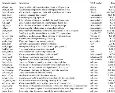
evapotranspira-Table 1.Precipitation Runoff Modeling System (PRMS) calibration parameters used in this study. The values in the column labeled “PRMS module” identify the module type equation(s) from the PRMS source code (see Markstrom et al., 2015).

Parameter name Description PRMS module Range

adjmix_rain Factor to adjust rain proportion in a mixed rain/snow event climate 0.6–1.4 tmax_allrain Maximum air temperature above which precipitation is rain climate −8.0–60.0 tmax_allsnow Maximum air temperature below which precipitation is snow climate −10.0–40.0

dday_intcp Intercept in degree–day equation solar radiation −60.0–10.0

dday_slope Slope in degree–day equation solar radiation 0.2–0.9

ppt_rad_adj Solar radiation adjustment threshold for precipitation days solar radiation 0.0–0.5 radj_sppt Solar radiation adjustment on summer precipitation days solar radiation 0.0–1.0 radj_wppt Solar radiation adjustment on winter precipitation days solar radiation 0.0–1.0 radmax Maximum solar radiation due to atmospheric effects solar radiation 0.1–1.0 tmax_index Temperature to determine precipitation adjustments to solar radiation solar radiation −10.0–110.0 jh_coef Coefficient used in Jensen–Haise potential ET computations Potential ET 0.005–0.06 jh_coef_ hru Coefficient used in Jensen–Haise potential ET computations Potential ET 5.0–25.0

srain_intcp Summer rain interception storage capacity interception 0.0–1.0

wrain_intcp Winter rain interception storage capacity interception 0.0–1.0

cecn_coef Convection condensation energy coefficient snow 2.0–10.0

emis_noppt Average emissivity of air on days without precipitation snow 0.757–1.0

freeh2o_cap Free-water holding capacity of snowpack snow 0.01–0.2

potet_sublim Snow sublimation fraction of potential ET snow 0.1–0.75

carea_max Maximum area contributing to surface runoff surface runoff 0.0–1.0

smidx_coef Non-linear contributing area coefficient surface runoff 0.001–0.06

smidx_exp Exponent in non-linear contributing area coefficient surface runoff 0.1–0.5 fastcoef_lin Linear coefficient in equation to route preferential-flow soil-zone 0.001–0.8 fastcoef_sq Non-linear coefficient in equation to route preferential-flow soil-zone 0.001–1.0 pref_flow_den Fraction of the soil zone in which preferential flow occurs soil-zone 0.0–0.1 sat_threshold Water capacity between field capacity and total saturation soil-zone 1.0–999.0

slowcoef_lin Linear coefficient for interflow routing soil-zone 0.001–0.5

slowcoef_sq Non-linear coefficient for interflow routing soil-zone 0.001–1.0

soil2gw_max Maximum soil water excess that is routed directly to groundwater soil-zone 0.0–0.5 soil_moist_max Maximum available water holding capacity of soil zone soil-zone 0.001–10.0 soil_rechr_max Maximum available water holding capacity of recharge zone soil-zone 0.001–5.0 ssr2gw_exp Non-linear coefficient in equation used to route soil-zone water to groundwater soil-zone 0.0–3.0 ssr2gw_rate Linear coefficient in equation used to route soil-zone water to groundwater soil-zone 0.05–0.8 transp_tmax Temperature that determines start of the transpiration period soil-zone 0.0–1000.0

gwflow_coef Linear groundwater discharge coefficient groundwater 0.001–0.5

tion lost from canopy interception, snow sublimation, and soil and plant losses from the root zone; (6) interflow (ss-res_flow) – shallow lateral flow in the unsaturated zone to the connected stream segment; (7) baseflow (gwres_flow) – the component of flow from the saturated zone to the connected stream segment; and (8) runoff (hru_outflow) – the total flow from the HRU contributing to streamflow in the connected stream segment. It is assumed that these eight output vari-ables are representative of the processes typically considered in hydrological studies with DPHMs. Details of how these processes are simulated by PRMS are described by Mark-strom et al. (2015).

2.4 Performance statistics

For DPHMs, there are many different performance measures that have been developed for different purposes (Krause et

“flashi-ness”, and day-to-day timing, respectively. These perfor-mance statistics are computed on the daily time series of the process variables for the 10-year evaluation period.

2.5 FAST analysis

Parameter sensitivity analysis measures the variability of model output given variability of calibration parameter val-ues. This is determined by partitioning the total variabil-ity in the model output or change in performance statistics to individual calibration parameters (Reusser et al., 2011). The Fourier amplitude sensitivity test (FAST) (Schaibly and Shuler, 1973; Cukier et al., 1973, 1975; Saltelli et al., 2006) was selected for this study because it has been demonstrated that it can efficiently estimate non-linear hydrologic model parameter sensitivity (Guse et al., 2014; Pfannerstill et al., 2015; Reusser et al., 2011). FAST is a variance-based global sensitivity algorithm that estimates the first-order partial vari-ance of model output explained by each calibration parame-ter (hereafparame-ter referred to as parameter sensitivity). Specifi-cally, this first-order variance is the variability in the output that is directly attributable to variations in any one parameter and is distinguishable from higher order variances associated with parameter interactions. An important caveat is that these higher order variances are not accounted for in the analysis. It is assumed that first-order partial variance is sufficient to identify sensitive parameters. This same assumption, as ap-plied to process identification, may be more problematic. If there are sets of interactive sensitive parameters that have not been identified, then the associated process(es) will not be identified as such.

Selected parameters are varied within defined ranges at in-dependent frequencies among different model runs. FAST identifies the variability of parameter sensitivities and their ranks, by means of their contribution to total power in the power spectrum. FAST has been implemented as the ‘fast’ library in the statistical software R (Reusser et al., 2011; Reusser, 2013; R Core Team, 2015) in two parts. In the first part, the user identifies the calibration parameters and respec-tive value ranges for the test, then FAST generates sets of test calibration parameter values (hereafter referred to astrials). Calibration parameter values are varied across the trials ac-cording to non-harmonic fundamental frequencies. The user then runs the DPHM for each trial and computes correspond-ing performance statistics. Then the user runs the second part of the FAST package that performs a Fourier analysis of the performance statistics over the trial space looking for the fre-quency signatures associated with each calibration parame-ter.

The FAST methodology results in a simple procedure for computing parameter sensitivities on an HRU basis for all the CONUS. The steps in this process are as follows:

1. Assign appropriate ranges for the 35 calibration param-eters (Markstrom et al., 2015; as in LaFontaine et al., 2013). These are shown in Table 1.

2. Run the first part of the FAST procedure (as described above) to develop over 9000 unique parameter sets, comprised of value combinations for the calibration pa-rameters. The total number and content of these parame-ter sets, and the results from their simulation by PRMS, are completely determined by the first part of the FAST procedure in order to investigate the trial space. Each of the prescribed simulations are independent of each other so they can run in parallel on a computer cluster. 3. Compute the FDSS based performance statistics (mean,

CV, and AR-1) for each process.

4. Run the second part of the FAST procedure (as de-scribed above) using output from step 3, resulting in PRMS parameter sensitivities, at each HRU, for the 56 combinations of seven performance statistics and eight processes (plus totals).

3 Results

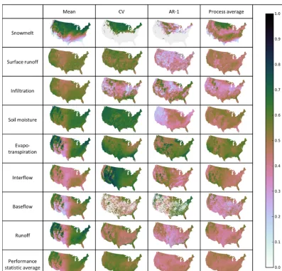
3.1 Parameter sensitivity by process and performance statistic

Figure 2.Maps of the conterminous US showing Precipitation–Runoff Modeling System parameter sensitivity by Hydrologic Response Unit (HRU) by process and performance statistic. The HRU parameter sensitivity is computed by summing the first-order sensitivity for all parameters. The process average maps are made by averaging the parameter sensitivity values computed for the different performance statistics. The performance statistic maps are made averaging the parameter sensitivity values computed for the different processes.

the largest sum on an HRU is referred to as thedominant pro-cessfor that HRU.

An example of an inferior process is clearly seen in the case of the mean of the snowmelt process in the southern CONUS HRUs. This is because the occurrence of snow in these areas is very infrequent. Also, there were HRUs for which the value of some performance statistics were mathe-matically undefined for certain processes (e.g., AR-1 and CV for the baseflow and snowmelt processes). These cases occur when the output variable representing the process does not change at all through time, regardless of the parameter val-ues, and are extreme examples of inferior processes. Like-wise, a clear example of a dominant hydrologic process is the CV of interflow in the Intermountain West region of the CONUS (Figs. 1 and 2). This means that for these HRUs,

there exist some calibration parameters that can be varied, which affect this process to a very high degree.

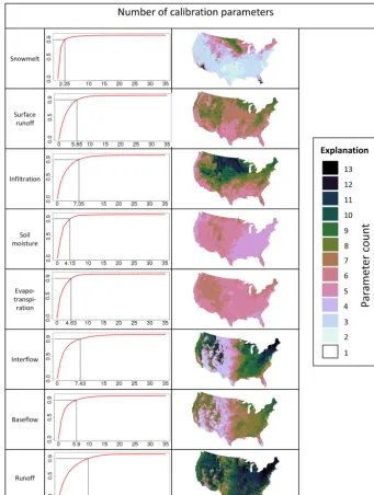
Figure 3.Cumulative parameter sensitivity across all Hydrologic Response Units (HRUs) in the CONUS Precipitation–Runoff Modeling System application are shown by process. (a)–(h)show the parameter count necessary to account for 90 % of the cumulative parameter sensitivity, summarized across all HRUs. For this count, the parameters are ranked and summed until the 90 % level is reached. The maps

(i)–(p)show the count of ranked parameters required to reach the 90 % level on an HRU-by-HRU basis, by process.

the ability of any parameter(s) to change the total volume of water during a simulation, seems to have a low sensitiv-ity band in the Great Plains region for all processes except for snowmelt (Fig. 1). This band of low sensitivity has been noted in other modeling studies (Newman et al., 2015; Bock et al., 2016).

3.2 Parameter count required to parameterize each process

cumula-tive sensitivity is plotted for the parameter in rank 2, and so on, until the cumulative sensitivity of all 35 calibration pa-rameters is accounted for. The plots in Fig. 3a–h show that far fewer than the full 35 parameters are needed to account for most of the parameter sensitivity. In fact, to account for 90 % of the parameter sensitivity, this count varies from a low value of just over two for snowmelt to an average high value of over nine for runoff in selected HRUs.

The actual count of calibration parameters required to ac-count for 90 % of the parameter sensitivity varies by pro-cess and region, as shown by the maps in Fig. 3i–p. These maps were generated by counting the number of parameters required to obtain the 90 % cumulative sensitivity level for each HRU. For example, Fig. 3o indicates that for the base-flow process, between three and nine parameters are needed to account for 90 % of the parameter sensitivity in the vari-ous HRUs across the CONUS, with the higher count needed in mountainous, Great Lakes, and New England regions. The maps also indicate that between 2 (Fig. 3i) and 13 parame-ters (Fig. 3k, n, and p) are required for parameterization of these processes. This analysis indicates that more parameters are needed to simulate the components of streamflow (e.g., baseflow, interflow, and surface runoff) than processes that do not result directly in flow (e.g., snowmelt, evapotranspi-ration, and soil moisture). In addition, simulated processes that are identified as being sensitive to parameters with which they are not normally associated, may indicate that these pro-cesses are a convolution of other propro-cesses, consequently making parameters sensitive that are not normally sensitive.

Visually, these maps (Fig. 3i–p) indicate that HRU calibra-tion parameter counts vary regionally. For most processes, higher parameter counts are seen in the more mountainous regions of the Cascade, Sierra Nevada, Rocky, Ozark, and Appalachian mountains, although this is true to a much lesser extent for the evapotranspiration and soil moisture processes (Fig. 3m and l). Higher values also seem prevalent in the New England and Great Lake regions (Fig. 1). This result seems to indicate that, no matter which part of the hydrologic cycle is simulated, more parameters are required in these regions. In contrast, low parameter counts seem prevalent in the Great Plains and Desert Southwest regions.

Finally, Fig. 3 illustrates the extent to which it is possi-ble to decompose the parameter estimation propossi-blem into a sub-set of independent problems, and hence reduce the di-mensionality of the inference problem and avoid the trou-blesome nature of parameter interactions. By considering a single (or reduced set of) processes and performance statis-tic categories at a time, the sensitive parameter space can be substantially reduced. It also illustrates that there is a strong spatial component to this decomposition. In order to make the information presented in Fig. 3 more useful for DPHM application, the particular sensitive parameters have been de-termined for each HRU by ranking the calibration param-eters by sensitivity for each category of process and per-formance statistic for each individual HRU and is

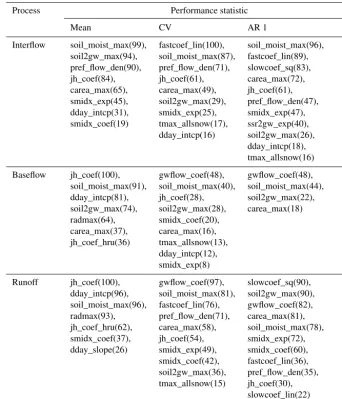
summa-rized by counting the occurrence of each parameter across the HRUs and ranking them within their respective category of process and performance statistic (Table 2). To address the issue of the spatial variability of these parameters, the per-centage of the total number of HRUs for which that param-eter is sensitive is shown as the number in parentheses af-ter the parameaf-ter name in Table 2. Higher percentage values would indicate that the corresponding parameter is sensitive across more of the CONUS. Refer to Table 1 for a complete description of these parameters.

When looking at the categorical parameter lists of Table 2, it is expected that different parameters would associate with different processes (i.e., along a column), but it is surpris-ing to see how different the parameter lists are for different performance statistics (moving across a row) for the same process. An example of this is the baseflow process: the base-flow coefficient (PRMS parameter gwbase-flow_coef) is the most sensitive parameter for performance statistics CV and AR-1, but is not even in the list of sensitive parameters for the per-formance statistics related to the mean of the process. This implies that this parameter is influential for affecting the tim-ing of baseflow, while it does not have any effect on the total volume of baseflow.

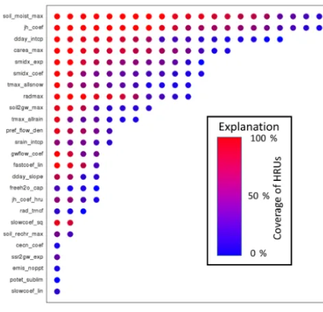
Further inspection of Table 2 indicates that some calibra-tion parameters occur in many of the 24 categories (8 pro-cesses times 3 performance statistics), while some parame-ters do not occur at all. A count of how many times each parameter occurs provides insight into how many process and/or performance statistic combinations that particular pa-rameter influences. To investigate this for the CONUS appli-cation, another view of the information in Table 2 is shown in Fig. 4. The 25 sensitive calibration parameters from Ta-ble 2 are listed on theyaxis of Fig. 4, ranked by order of the number of times that they appear in the process and/or per-formance statistic categories. Furthermore, each appearance is indicated by an adjacent circle. Independent of the num-ber of times a parameter occurs within a category (numnum-ber of circles), the color of the circle visually indicates the propor-tion of the CONUS HRUs that are affected by that param-eter. Specifically, a red circle indicates that more HRUs are affected, while blue indicates that fewer HRUs are affected.

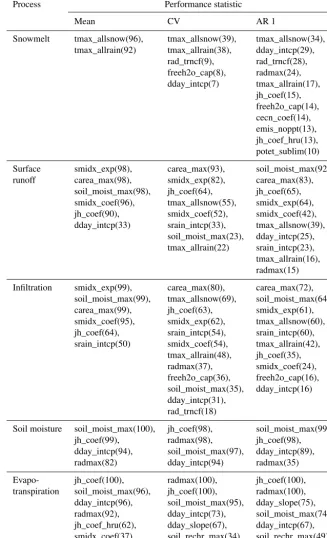
Table 2.Ordered list of most sensitive Precipitation–Runoff Modeling System calibration parameters by process and performance statistic. The parameters listed in each cell of the table are those that are required to account for 90 % of the cumulative sensitivity across all hydrologic response units (HRUs). The number in parentheses following the parameter name is the proportion of the CONUS HRUs, in percent, in which that parameter is part of the set that accounts for 90 % of the cumulated sensitivity on an HRU-by-HRU basis. These parameters are described in Table 1.

Process Performance statistic

Mean CV AR 1

Snowmelt tmax_allsnow(96), tmax_allsnow(39), tmax_allsnow(34), tmax_allrain(92) tmax_allrain(38), dday_intcp(29),

rad_trncf(9), rad_trncf(28), freeh2o_cap(8), radmax(24), dday_intcp(7) tmax_allrain(17),

jh_coef(15), freeh2o_cap(14), cecn_coef(14), emis_noppt(13), jh_coef_hru(13), potet_sublim(10)

Surface smidx_exp(98), carea_max(93), soil_moist_max(92), runoff carea_max(98), smidx_exp(82), carea_max(83),

soil_moist_max(98), jh_coef(64), jh_coef(65), smidx_coef(96), tmax_allsnow(55), smidx_exp(64), jh_coef(90), smidx_coef(52), smidx_coef(42), dday_intcp(33) srain_intcp(33), tmax_allsnow(39),

soil_moist_max(23), dday_intcp(25), tmax_allrain(22) srain_intcp(23), tmax_allrain(16), radmax(15)

Infiltration smidx_exp(99), carea_max(80), carea_max(72), soil_moist_max(99), tmax_allsnow(69), soil_moist_max(64), carea_max(99), jh_coef(63), smidx_exp(61), smidx_coef(95), smidx_exp(62), tmax_allsnow(60), jh_coef(64), srain_intcp(54), srain_intcp(60), srain_intcp(50) smidx_coef(54), tmax_allrain(42),

tmax_allrain(48), jh_coef(35), radmax(37), smidx_coef(24), freeh2o_cap(36), freeh2o_cap(16), soil_moist_max(35), dday_intcp(16) dday_intcp(31),

rad_trncf(18)

Soil moisture soil_moist_max(100), jh_coef(98), soil_moist_max(99), jh_coef(99), radmax(98), jh_coef(98), dday_intcp(94), soil_moist_max(97), dday_intcp(89), radmax(82) dday_intcp(94) radmax(35)

Evapo- jh_coef(100), radmax(100), jh_coef(100), transpiration soil_moist_max(96), jh_coef(100), radmax(100),

Table 2.Continued.

Process Performance statistic

Mean CV AR 1

Interflow soil_moist_max(99), fastcoef_lin(100), soil_moist_max(96), soil2gw_max(94), soil_moist_max(87), fastcoef_lin(89), pref_flow_den(90), pref_flow_den(71), slowcoef_sq(83), jh_coef(84), jh_coef(61), carea_max(72), carea_max(65), carea_max(49), jh_coef(61), smidx_exp(45), soil2gw_max(29), pref_flow_den(47), dday_intcp(31), smidx_exp(25), smidx_exp(47), smidx_coef(19) tmax_allsnow(17), ssr2gw_exp(40),

dday_intcp(16) soil2gw_max(26), dday_intcp(18), tmax_allsnow(16)

Baseflow jh_coef(100), gwflow_coef(48), gwflow_coef(48), soil_moist_max(91), soil_moist_max(40), soil_moist_max(44), dday_intcp(81), jh_coef(28), soil2gw_max(22), soil2gw_max(74), soil2gw_max(28), carea_max(18) radmax(64), smidx_coef(20),

carea_max(37), carea_max(16), jh_coef_hru(36) tmax_allsnow(13),

dday_intcp(12), smidx_exp(8)

Runoff jh_coef(100), gwflow_coef(97), slowcoef_sq(90), dday_intcp(96), soil_moist_max(81), soil2gw_max(90), soil_moist_max(96), fastcoef_lin(76), gwflow_coef(82), radmax(93), pref_flow_den(71), carea_max(81), jh_coef_hru(62), carea_max(58), soil_moist_max(78), smidx_coef(37), jh_coef(54), smidx_exp(72), dday_slope(26) smidx_exp(49), smidx_coef(60),

smidx_coef(42), fastcoef_lin(36), soil2gw_max(36), pref_flow_den(35), tmax_allsnow(15) jh_coef(30),

slowcoef_lin(22)

Parameters adjmix_rain, fastcoef_sq, ppt_rad_adj, radj_sppt, radj_wppt, sat_threshold , not sensitive ssr2gw_rate, tmax_index, transp_tmax, wrain_intcp

unintended parameter interaction during calibration. Ideally, these parameters could be estimated from reliable external data, set for the model and not calibrated. The parameters that affect the least number of process categories (aside from the parameters that are never sensitive) are cecn_coef (con-vection condensation energy coefficient), ssr2gw_exp (co-efficient in equation used to route water from the soil to the groundwater reservoir), emis_noppt (emissivity of air on days without precipitation), potet_sublim (fraction of poten-tial evapotranspiration that is sublimated), and slowcoef_lin (slow interflow routing coefficient). Ideally, these parameters could be set to default values since there is limited value in calibrating them.

Also apparent from Fig. 4 is that there are many param-eters between these two extreme groups. Paramparam-eters like smidx_coef (soil moisture index for contributing area

Figure 4.Summarizes the frequency of occurrence of the different calibration parameters in the process and/or performance statistic categories of Table 2. The circles in each row adjacent to a parame-ter name indicate how many times the respective parameparame-ter occurs in these different categories. Parameters with more circles are af-fecting more process categories. The color of each circle indicates the extent of the spatial coverage of that occurrence; specifically, red circles (as opposed to blue) indicate that more Hydrologic Re-sponse Units are affected by the respective parameter.

3.3 Identification of dominant and inferior processes by HRU

To identify the dominant and inferior process(es) by geo-graphic area, the following procedure is done for each HRU: 1. the parameter sensitivity scores are summed for each parameter, resulting in a score for each parameter for each time-series output variable and performance statis-tic;

2. the parameter scores are averaged by performance statistics, resulting in a score for each process;

3. the process scores are ranked for each HRU;

4. the top (and bottom) ranked process determines the most dominant (and most inferior) single process for each HRU as shown in Fig. 5.

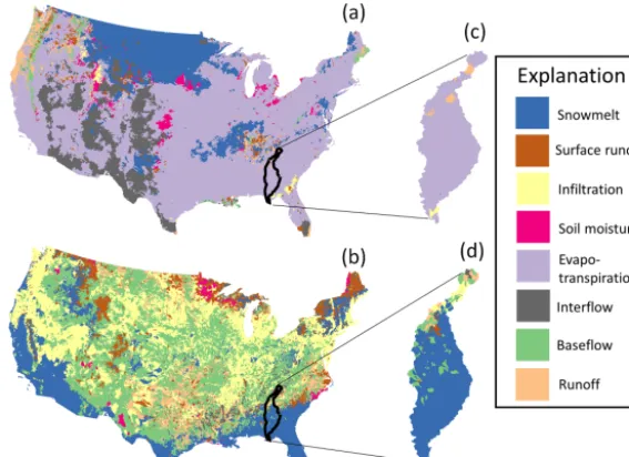
Generally, Fig. 5a shows that evapotranspiration is the most prevalent dominant process for the CONUS. This is proba-bly because it is a major component of the hydrologic cycle and sensitive parameters are available to affect it in every HRU. However, this is not universal, and the dominant pro-cess varies by geographic region, with snowmelt being the

dominant process in the northern Great Planes and northern Rocky Mountains, total runoff being the most important in the Pacific Northwest, and with interflow important in bands across the Intermountain West (Fig. 1). Each process is dom-inant somewhere depending on local conditions. Equally in-formative are the locations of the most inferior processes (Fig. 5b). This clearly shows that PRMS snowmelt param-eters are not sensitive across the Central Valley of Califor-nia, and in the Deep South and the southwestern US (Fig. 1). Areas where runoff is more dominant than evapotranspira-tion, as in the Cascade Mountains and coastal areas of the Pacific Northwest, are locations where the runoff is a sub-stantially greater part of the water budget. Interestingly, infil-tration and baseflow appear to be equally inferior across most of CONUS, with pockets of HRUs that are insensitive to soil moisture, surface runoff, and interflow, depending on local conditions. There are no HRUs that rank evapotranspiration as the most inferior process.

Dominant and inferior processes can be identified for HRUs at the watershed scale as well. Figure 5c shows the most dominant process by HRU for the Apalachicola– Chattahoochee–Flint River watershed in the southeast-ern US. This watershed has been the subject of previous PRMS modeling studies (LaFontaine et al., 2013). When us-ing this information at a finer resolution, it shows that evap-otranspiration is the most dominant process watershed wide, but with pockets of HRUs in the northern part of the wa-tershed where runoff is the most dominant and a pocket in the southern part of the watershed where infiltration is most dominant. Likewise, the most inferior process for each HRU is identified in Fig. 5d. This clearly indicates that parame-ters and performance statistics related to snowmelt, and to a lesser degree baseflow, do not need to be considered when modeling this watershed. Figure 5d also indicates that in the northern part of the watershed, infiltration and runoff are in-ferior processes as well, which could in part be due to imper-vious conditions around the Atlanta metropolitan area.

4 Discussion

4.1 Causes of parameter sensitivity

There are regions where parameter sensitivity is typically high for a particular performance statistic (e.g., New England region (Fig. 1) for performance statistic based on mean of processes) or typically low (e.g., Great Plains region (Fig. 1) for mean of processes) regardless of the process (Fig. 2). Why do the HRUs of some regions exhibit parameter sensi-tivity to almost all processes, while others exhibit parameter sensitivity to almost none? All other things being equal, there can only be two sources of these spatial patterns:

Figure 5.Precipitation–Runoff Modeling System parameter sensitivity organized by process ranked for each hydrologic response unit for the entire conterminous US – maps(a)and(b)– and for the Apalachicola–Chattahoochee–Flint River Basin – maps(c)and(d). The maps on the top(a, c)show the most dominant process, while the maps on the bottom(b, d)show the most inferior process.

A theoretical example of this could be if an HRU is char-acterized as entirely impervious, resulting in the non-existence of any simulated soil water.

2. Patterns in the climate data used to drive the model (e.g., daily temperature and precipitation) could control model response. A theoretical example of this could be an HRU that receives no precipitation.

The hydrologic response of the HRUs in either case would always remain unchanged, regardless of changes in any pa-rameter value. In either case, these sources of information are independent of the DPHM and could lead to the conclusion that the dominant processes identified by the methods out-lined in this article could correspond to perceptible dominant processes in the physical world (i.e., how the “real world” works).

The number of unique calibration parameters for each pro-cess in Table 2 (i.e., counting the parameters across each row) may provide some insight into the complexity of each pro-cess as represented in the model structure of PRMS. In the-ory, more “complicated” hydrologic processes would require more parameters for parameterization than the “simpler” ones. According to this view, runoff (16 calibration param-eters), infiltration (12 calibration paramparam-eters), and interflow (12 calibration parameters) are the most complex processes to simulate, with soil moisture (4) being the simplest. Base-flow (11 calibration parameters), snowmelt (11 calibration parameters), surface runoff (10 calibration parameters), and evapotranspiration (8 calibration parameters) are in between. This reflects the fact that in PRMS, runoff is a much more complicated calculation with many of the other processes

di-rectly contributing information. Also apparent is that more parameters are needed to simulate the components of stream-flow (e.g., basestream-flow, interstream-flow, and surface runoff) than pro-cesses that do not result directly in flow (e.g. snowmelt, evap-otranspiration, and soil moisture). The only process that does not follow this pattern is infiltration. Storm-event-based infil-tration is typically simulated with sub-daily time steps to ac-count for the variability of time and intensity in this process. It is possible that PRMS must compensate for this shortcom-ing in structure with a more complex parameterization of the process.

alter-native or improved performance statistics could resolve this issue.

4.2 Choice of performance statistic

The maps of Fig. 2 clearly illustrate the importance that choice of performance statistic can make in terms of evalua-tion of hydrologic response. When the maps of performance statistics within a single hydrologic process are compared (i.e., the maps across a single row), the spatial patterns and magnitude of the parameter sensitivity can be very different. This could indicate that the performance statistics based on the FDSS truly are non-redundant and are accounting for dif-ferent aspects of the processes.

Table 2 indicates that the baseflow coefficient (PRMS pa-rameter gwflow_coef, Markstrom et al., 2015) is the most sensitive parameter for performance statistics CV and AR-1, but not sensitive to the mean of the baseflow process perfor-mance statistics. This points to the fact that despite having knowledge of a parameter being associated with the compu-tation of a certain process, sensitivity analysis can reveal that the response of the simulation is completely different when the performance statistic changes. It also indicates that sen-sitivity analysis might be an important step in selection of an appropriate performance statistic and that uncritical applica-tion of performance statistics may be misleading.

4.3 Spatial aspects of dominant and inferior processes

When the dominant and inferior processes are determined for an HRU (Fig. 5), it is possible that certain parameters are included in both the most dominant and most inferior pro-cesses at the same time. This apparent contradiction is not necessarily a conflict but indicates that the calibration pa-rameters must work in concert with the evaluation method. For example, there exist HRUs where the evapotranspiration process is dominant and at the same time the runoff or infil-tration processes are inferior (Fig. 5a and b). The parameter soil_moist_max is indicated as being sensitive for all three of these processes (Table 2). This parameter would demon-strate equifinality if evaluated within the context of the infe-rior processes (i.e., those output variables and performance statistics associated with the inferior process) but would be a very effective calibration parameter resulting in optimal val-ues when viewed within the context of parameters and vari-ables of the dominant process.

This method of identification of inferior and dominant pro-cesses for a specific geographical location (i.e., HRU, water-shed, or region), determined by sensitivity analysis, is de-fined within the context of the application of the DPHM and may not necessarily have the same meaning within a differ-ent context. However, this methodology does have the ability to spatially classify watersheds and identify dominant pro-cesses. This classification scheme depends not only on the physiographic nature of the watershed, but also on the scale,

resolution, and purpose that were considered by the modeler when the application was developed.

4.4 Further study

Providing modelers with reduced lists of calibration pa-rameters on an HRU-by-HRU, watershed-by-watershed, or region-by-region basis is the first step in the path of this re-search. Subsequent steps to this approach could be devel-oped into more sophisticated methods where orthogonal out-put variables and performance statistics could provide much more insight into methods of effective model calibration. Other advancements in this approach may identify groups of parameters that effectively behave together, thus reducing the number of parameters and making specific model output respond more directly to a single or a few parameters, reduc-ing parameter interaction. This suggests that model parame-terization and calibration might benefit from a step-by-step strategy, using as much information as possible to set non-interactive parameters and remove them from consideration before the more interactive parameters are calibrated, reduc-ing the dimensionality of the problem (Hay et al., 2006; Hay and Umemoto, 2006).

Another question for future research is: Does the classi-fication of dominant hydrologic processes, both geographi-cal and categorigeographi-cal, as described in this study, apply in other contexts? Comparable findings from other modeling studies, such as those by Newman et al. (2015) and Bock et al. (2016), might indicate that there could be a connection. These other studies use the same input information (i.e., being driven with the same climate data and using the same sources of information for parameter estimation), and thus simulation results and model sensitivity to this information might be similar. Also, can real world watersheds be classified by sen-sitivity analysis using DPHMs? Based on the findings of the work presented so far, the answer is inconclusive. Clearly there are some results that indicate that it might be possible. For example, the methods described here effectively identify “snowmelt watersheds” in the mountainous and northern lat-itudes, but, is all of this necessary to accomplish this? Might simpler methods (e.g., an isohyetal snowfall map) identify snowmelt watersheds just as effectively?

pa-rameters. Future work might be to determine the effect of us-ing different modules or maybe even to determine the selec-tion of the PRMS modules through sensitivity analysis. Just as the spatial and temporal scope of any modeling project must be defined, the scope of the hydrologic processes, and the detail to which these processes are simulated, must be likewise defined. Also, alternative ways of defining HRUs (e.g., larger or smaller, or even based on dominant process in-stead of geographic location) could affect the analysis. Model development and application could perhaps proceed by first accounting for those factors that have the most effect.

5 Conclusion

Watersheds in the real world clearly exhibit hydrologic be-havior determined by dominant processes based on geo-graphic location (i.e., land surface conditions and climate forcings). A methodology has been developed to identify re-gions, watersheds, and HRUs according to dominant pro-cess(es) on the basis of parameter sensitivity response with respect to a distributed-parameter hydrology model. The pa-rameters in this model were divided into two groups – those that are used for model calibration and those that were not. A global parameter sensitivity analysis was performed on the calibration parameters for all HRUs derived for the contermi-nous US. Categories of parameter sensitivity were developed in various ways, on the basis of geographic location, hydro-logic process, and model response. Visualization of these cat-egories provides insight into model performance, and useful information about how to structure the modeling application should take advantage of as much local information as pos-sible.

By definition, an insensitive parameter is one that does not affect the output. Ideally, a distributed-parameter hydrology model would have just a few calibration parameters, all of them meaningful, each controlling the algorithms related to the corresponding process. This would result in low parame-ter inparame-teraction and a clear correspondence between input and output. However, this is not always the case, and despite the fact that parameter interaction is unavoidable in these types of models, this behavior is also seen in the real world. For instance, in watersheds where evaporation is very high, an-tecedent soil moisture is affected, which has a direct influ-ence on infiltration. The real world process of evaporation has an effect on infiltration, just as evaporation parameters have an effect on simulation of infiltration in watershed hy-drology models. Application of distributed-parameter hydro-logic modeling application require that the uncertainty prob-lem and the calibration probprob-lem be addressed at the same time. While the user of a DPHM can do nothing about the complexity of the model’s internal structure, the apparent complexity can be reduced by limiting the parameters and the affected output under consideration.

Results of this study indicate that it is possible to identify the influence of different hydrologic processes when simu-lating with a distributed-parameter hydrology model on the basis of parameter sensitivity analysis. Factors influencing this analysis include geographic area, topography, land cover, soil, geology, climate, and other unidentified physical effects. Identification of these processes allows the modeler to focus on the more important aspects of the model input and out-put, which can simplify all facets of the hydrologic modeling application.

6 Data availability

The Precipitation–Runoff Modeling System software used in this study is developed, documented, and distributed by the US Geological Survey. It is in the public domain and freely available from their web site (http://wwwbrr.cr.usgs.gov/ prms). Data analysis and plotting is done with the R software package (http://www.r-project.org), which is freely available, subject to the GNU General Public License.

The climate forcing data set used in this study came from the US Geological Survey Geo Data Portal (http://cida.usgs.gov/climate/gdp). The HRU delineation and default parameterization came from the US Geo-logical Survey GeoSpatial Fabric (http://wwwbrr.cr.usgs. gov/projects/SW_MoWS/GeospatialFabric.html). Finally, the parameter sensitivity output values that were used to make the maps and tables in this article are available at ftp://brrftp.cr.usgs.gov/pub/markstro/hess.

Edited by: E. Zehe

Reviewed by: S. Höllering and B. Guse

References

Ali, G., Tetzlaff, D., Soulsby, C., McDonnell, J. and Capell, R.: A comparison of similarity indices for catchment classification using a cross-regional dataset, Adv. Water Resour., 40, 11–22, doi:10.1016/j.advwatres.2012.01.008, 2012.

Amorocho, J. and Hart, W. E.: A critique of current methods in hydrologic systems investigation, Trans. Am. Geophys. Un., 45, 307–321, 1964.

Archfield, S. A., Kennen, J. G., Carlisle, D. M., and Wolock, D. M.: An objective and parsimonious approach for classifying nature flow regimes at a continental scale, River Res. Appl., 30, 1166– 1183, 2014.

Battaglin, W. A., Hay, L. E., and Markstrom, S. L.: Simulating the potential effects of climate change in two Colorado Basins and at two Colorado ski areas, Earth Interact., 15, 1–23, 2011. Beven, K., Changing ideas in hydrology – The case of

physically-based models, J. Hydrol., 105, 157–172, 1989.

Beven, K: A manifesto for the equifinality thesis, J. Hydrol., 320, 18–36, doi:10.1016/j.jhydrol.2005.07.007, 2006.

wa-ter balance model for the conwa-terminous United States, Hy-drol. Earth Syst. Sci., 20, 2861–2876, doi:10.5194/hess-20-2861-2016, 2016.

Bower, D. E.: Evaluation of the Precipitation-Runoff Modeling System, Beaver Creek, Kentucky, US Geological Survey Scien-tific Investigations Report 84-4316, US Geological Survey, 1–39, 1985.

Boyle, D. P., Lamorey, G. W., and Huggins, A. W.: Application of a hydrologic model to assess the effects of cloud seeding in the Walker River basin, Nevada, J. Weather Modificat., 38, 66–67, 2006.

Brun, R., Reichert, P., and Kunsch, H. R.: Practical identifiability analysis of large environmental simulation models, Water Re-sour. Res., 37, 1015–1030, doi:10.1029/2000wr900350, 2001. Cary, L. E.: Techniques for estimating selected parameters of the

U.S. Geological Survey’s Precipitation-Runoff Modeling System in eastern Montana and northeastern Wyoming, US Geological Survey Water-Resources Investigations Report 91-4068, US Ge-ological Survey, Reston, Virgina, 1–39, 1991.

Chaney, N. W., Herman, J. D., Reed, P. M., and Wood, E. F.: Flood and drought hydrologic monitoring: the role of model pa-rameter uncertainty, Hydrol. Earth Syst. Sci., 19, 3239–3251, doi:10.5194/hess-19-3239-2015, 2015.

Clark, M. P. and Vrugt, J. A.: Unraveling uncertainties in hydrologic model calibration: Addressing the problem of compensatory parameters, Geophys. Res. Lett., 33, L06406, doi:10.1029/2005gl025604, 2006.

Cukier, R. I., Fortuin, C. M., and Shuler, K. E.: Study of the sensi-tivity of coupled reaction systems to uncertainties in rate coeffi-cients I, J. Chem. Phys., 59, 3873–3878, 1973.

Cukier, R. I., Schaibly, J. H., and Shuler, K. E.: Study of the sensi-tivity of coupled reaction systems to uncertainties in rate coeffi-cients III, J. Chem. Phys., 63, 1140–1149, 1975.

Cuntz, M., Mai, J., Zink, M., Thober, S., Kumar, R., Schafer, D., Schron, M., Craven, J., Rakovec, O., Spieler, D., Prykhodko, V., Dalmasso, G., Musuuza, J., Langenberg, B., Attinger, S., and Samaniego, L.: Computationally inexpensive identification of noninformative model parameters by sequential screening, Wa-ter Resour. Res., 51, 6417–6441, doi:10.1002/2015WR016907, 2015.

Duan, Q., Schaake, J., Andréassian, V., Franks, S., Goteti, G., Gupta, H. V., Gusev, Y. M., Habets, F., Hall, A., Hay, L., Hogue, T., Huang, M., Leavesley, G., Liang, X., Nasonova, O. N., Noil-han, J., Oudin, L., Sorooshian, S., Wagener, T., and Wood, E. F.: Model Parameter Estimation Experiment (MOPEX): An overview of science strategy and major results from the second and third workshops, J. Hydrol., 320, 3–17, 2006.

Dudley, R. W.: Simulation of the quantity, variability, and tim-ing of streamflow in the Dennys River Basin, Maine, by use of a precipitation-runoff watershed model, US Geological Survey Scientific Investigations Report 2008-5100, US Geological Sur-vey, Reston, Virgina, 1–44, 2008.

Ewan, J.: Hydrograph matching method for measur-ing model performance, J. Hydrol., 408, 178–187, doi:10.1016/j.jhydrol.2011.07.038, 2011.

Freeze, R. A. and Harlan, R. L.: Blueprint for a physically-based, digitally-simulated hydrologic response model, J. Hydrol., 9, 237–258, 1969.

Grayson, R. B., Moore, I. D., and McMahon, T. A.: Physically based hydrologic modeling, 2, Is the concept realistic?, Water Resour. Res., 28, 2659–2666, 1992.

Gupta, H. V., Wagener, T., and Liu, Y. Q.: Reconciling theory with observations: elements of a diagnostic approach to model eval-uation, Hydrol. Process., 22, 3802–3813, doi:10.1002/hyp.6989, 2008.

Gupta, H. V., Kling, H., Yilmaz, K. K., and Martinez, G. F.: Decom-position of the mean squared error and NSE performance criteria: Implications for improving hydrological modelling, J. Hydrol., 377, 80–91, doi:10.1016/j.jhydrol.2009.08.003. 2009.

Gupta, H. V., Clark, M. P., Vrugt, J. A., Abramowitz, G., and Ye, M.: Towards a comprehensive assessment of model structural adequacy, Water Resour. Res., 48, W08301, doi:10.1029/2011wr011044, 2012.

Guse, B., Reusser, D. E., and Fohrer, N.: How to improve the representation of hydrological processes in SWAT for a low-land catchment – Temporal analysis of parameter sensitiv-ity and model performance, Hydrol. Process., 28, 2651–2670, doi:10.1002/hyp.9777, 2014.

Hay, L. E., Leavesley, G. H., Clark, M. P., Markstrom, S. L., Viger, R. J., and Umemoto, M.: Step-wise, multiple-objective calibra-tion of a hydrologic model for a snowmelt-dominated basin, J. Am. Water Resour., 42, 891–900, 2006.

Hay, L. E., Markstrom, S. L., and Ward-Garrison, C. D.: Watershed-scale response to climate change through the 21st century for selected basins across the United States, Earth Interact., 15, 1– 37, 2011.

Hay, L. E. and Umemoto, M.: Multiple-objective stepwise calibra-tion using Luca, US Geological Survey Open-File Report 2006-1323, US Geological Survey, Reston, Virgina, 1–25, 2006. He, Y., Bardossy, A., and Zehe, E.: A catchment classification

scheme using local variance reduction method, J. Hydrol., 411, 140–154, 2011.

Hrachowitz, M., Fovet, O., Ruiz, O., Euser, T., Gharari, S., Nijzink, R., Freer, J., Savenije, H. H. G., and Gascuel-Odoux, C.: Process consistency in models: The importance of system signatures, ex-pert knowledge, and process complexity, Water Resour. Res., 50, 7445–7469, doi:10.1002/2014WR015484, 2014.

Jakeman, A. and Hornberger, G.: How much complexity is war-ranted in a rainfall-runoff model?, Water Resour. Res., 29, 2637– 2649, 1993.

Kirchner, J. W., Hooper, R. P., Kendall, C., Neal, C., and Leavesley, G. H.: Testing and validating environmental models, Sci. Total Environ., 183, 33–47, 1996.

Koczot, K. M., Markstrom, S. L., and Hay, L. E.: Effects of base-line conditions on the simulated hydrologic response to projected climate change, Earth Interact., 15, 1–23, 2011.

Krause, P., Boyle, D. P., and Bäse, F.: Comparison of different effi-ciency criteria for hydrological model assessment, Adv. Geosci., 5, 89–97, doi:10.5194/adgeo-5-89-2005, 2005.

Markstrom, S. L., Hay, L. E., Ward-Garrison, C. D., Risley, J. C., Battaglin, W. A., Bjerklie, D. M., Chase, K. J., Christiansen, D. E. Dudley, R. W., Hunt, R. J., Koczot, K. M., Mastin, M. C., Regan, R. S., Viger, R. J., Vining, K. C., and Walker, J. F.: In-tegrated watershed scale response to climate change for selected basins across the United States, US Geological Survey Scientific Investigations Report 2011-5077, US Geological Survey, Reston, Virginia, 1–143, 2012.

Markstrom, S. L., Regan, R. S., Hay, L. E., Viger, R. J., Webb, R. M. T., Payn, R. A., and LaFontaine, J. H.: PRMS-IV, the precipitation-runoff modeling system, version 4, book 6, chap. B7, US Geological Survey Techniques and Methods, US Geological Survey, Reston, Virgina, 1–158, doi:10.3133/tm6B7, 2015.

Mayer, D. G. and Butler, D. G.: Statistical validation, Ecol. Model., 68, 21–32, 1993.

McDonnell, J., Sivapalan, M., Vaché, K., Dunn, S., Grant, G., Hag-gerty, R., Hinz, C., Hooper, R., Kirchner, J., and Roderick, M.: Moving beyond heterogeneity and process complexity: a new vision for watershed hydrology, Water Resour. Res., 43, 6 pp., doi:10.1029/2006wr005467, 2007.

Mendoza, P. A., Clark, M. P., Barlage, M., Rajagopalan, B., Samaniego, L., Abramowitz, G. and Gupta H., Are we unneces-sarily constraining the agility of complex process-based models?, Water Resour. Res., 51, 716–728, doi:10.1002/2014WR015820, 2015a.

Mendoza, P. A., Clark, M. P., Mizukami, N., Newman, A. J., Bar-lage, M. E., Gutmann, D. Rasmussen, R. M., Rajagopalan, B., Brekke, L. D., and Arnold, J. R.: Effects of hydrologic model choice and calibration on the portrayal of climate change im-pacts, J. Hydrometeorol., 16, 762–780, 2015b.

Merz, R. and Blöschl, G.: Regionalisation of catchment model pa-rameters, J. Hydrol., 287, 95–123, 2004.

Newman, A. J., Clark, M. P., Sampson, K., Wood, A., Hay, L. E., Bock, A., Viger, R. J., Blodgett, D., Brekke, L., Arnold, J. R., Hopson, T., and Duan, Q.: Development of a large-sample watershed-scale hydrometeorological data set for the contiguous USA: data set characteristics and assessment of regional variabil-ity in hydrologic model performance, Hydrol. Earth Syst. Sci., 19, 209–223, doi:10.5194/hess-19-209-2015, 2015.

Perrin, C., Michel, C., and Andreassian, V.: Does a large number of parameters enhance model performance? Comparative assess-ment of common catchassess-ment model structures on 429 catchassess-ments, J. Hydrol., 242, 275–301, doi:10.1016/s0022-1694(00)00393-0, 2001.

Pfannerstill, M., Guse, B., Reusser, D., and Fohrer, N.: Process verification of a hydrological model using a temporal parame-ter sensitivity analysis, Hydrol. Earth Syst. Sci., 19, 4365–4376, doi:10.5194/hess-19-4365-2015, 2015.

R Core Team: R: A language and environment for statistical com-puting, R Foundation for Statistical Comcom-puting, Vienna, Austria, http://www.R-project.org/ (last access: August 2015), 2015. Reusser, D. E.: Implementation of the Fourier amplitude

sensitiv-ity test (FAST), R package version 0.63, http://CRAN.R-project. org/package=fast (last access: August 2015), 2013.

Reusser, D. E. and Zehe, E.: Inferring model structural deficits by analyzing temporal dynamics of model performance and parameter sensitivity, Water Resour. Res., 47, W07550, doi:10.1029/2010WR009946, 2011.

Reusser, D. E., Buytaert, W., and Zehe, E.: Temporal dynamics of model parameter sensitivity for computationally expensive mod-els with the Fourier amplitude sensitivity test, Water Resour. Res., 47, W07551, doi:10.1029/2010WR009947, 2011. Saltelli, A., Ratto, M., and Tarantola, S.: Sensitivity analysis

prac-tices: strategies for model-based inference, Reliab. Eng. Syst. Saf., 10, 1109–1125, 2006.

Samaniego, L., Kumar, R., and Attinger, S.: Multiscale pa-rameter regionalization of a grid-based hydrologic model at the mesoscale, Water Resour. Res., 46, W05523, doi:10.1029/2008WR007327, 2010.

Sanadhya, P., Giron, J., and Arabi, M.: Global sensitivity analy-sis of hydrologic processes in major snow-dominated mountain-ous river basins in Colorado, Hydrol. Process., 28, 3404–3418, doi:10.1002/hyp.9896, 2013.

Schaefli, B. and Gupta, H. V.: Do Nash values have value?, Hydrol. Process., 21, 2075–2080, 2007.

Schaibly, J. H. and Shuler, K. E.: Study of the sensitivity of coupled reaction systems to uncertainties in rate coefficients II, applica-tions, J. Chem. Phys., 59, 3879–3888, 1973.

Seibert, J.: Regionalization of parameters for a conceptual rainfall-runoff model, Agr. Forest Meteorol., 98, 279–293, 1999. Sivakumar, B.: Dominant processes concept in hydrology: moving

forward, Hydrol. Process., 18, 2349–2353, 2004.

Sivakumar, B. and Singh, V. P.: Hydrologic system complex-ity and nonlinear dynamic concepts for a catchment classi-fication framework, Hydrol. Earth Syst. Sci., 16, 4119–4131, doi:10.5194/hess-16-4119-2012, 2012.

Sivakumar, B., Jayawardena, A. W., and Li, W. K.: Hydrologic com-plexity and classification: a simple data reconstruction approach, Hydrol. Process., 21, 2713–2728, 2007.

Thornton, P. E., Thornton, M. M., Mayer, B. W., Wilhelmi, N., Wei, Y., Devarakonda, R., and Cook, R. B.: Daymet: daily surface weather data on a 1-km grid for North America, version 2, data set, available at: http://daac.ornl.gov from Oak Ridge National Laboratory Distributed Active Archive Center, Oak Ridge, Ten-nessee, USA, doi:10.3334/ORNLDAAC/1219, 2014.

Viger, R. J.: Preliminary spatial parameters for PRMS based on the geospatial fabric, NLCD2001 and SSURGO, US Geological Sur-vey, Reston, Virgina, doi:10.5066/F7WM1BF7, 2014.

Viger, R. J. and Bock, A.: GIS features of the geospatial fabric for national hydrologic modeling, US Geological Survey, Reston, Virgina, doi:10.5066/F7542KMD, 2014.

Vogel, R. M.: Regional Calibration of Watershed Models, in: chap. 3 in Watershed Models, edited by: Singh, V. P. and Frevert, D. F., CRC Press, Boca Raton, Florida, 2005.

Wagener, T., McIntyre, N., Lees, M. J., Wheater, H. S., and Gupta, H. V.: Towards reduced uncertainty in conceptual rainfall–runoff modelling: dynamic identifiability analysis, Hydrol. Process., 17, 455–476, 2003.

Winter, T. C.: The concept of hydrologic landscapes, J. Am. Water Resour. Assoc., 37, 335–349, doi:10.1111/j.1752-1688.2001.tb00973.x, 2001.

Woods, R.: Seeing catchments with new eyes, Hydrol. Process., 16, 1111–1113, 2002.