www.hydrol-earth-syst-sci.net/20/3907/2016/ doi:10.5194/hess-20-3907-2016
© Author(s) 2016. CC Attribution 3.0 License.
Areal rainfall estimation using moving cars – computer experiments
including hydrological modeling
Ehsan Rabiei1, Uwe Haberlandt2, Monika Sester2, Daniel Fitzner2, and Markus Wallner3
1Institute of Water Resources Management, Hydrology and Agricultural Hydraulic Engineering, Leibniz University of
Hanover, 30167 Hanover, Germany
2Institute of Cartography and Geoinformatics, Leibniz University of Hanover, Hanover, Germany
3Federal Institute for Geosciences and Natural Resources, Groundwater Resources – Quality and Dynamics,
30655 Hanover, Germany
Correspondence to:Ehsan Rabiei ([email protected])
Received: 12 January 2016 – Published in Hydrol. Earth Syst. Sci. Discuss.: 9 February 2016 Revised: 24 July 2016 – Accepted: 31 August 2016 – Published: 26 September 2016
Abstract. The need for high temporal and spatial resolu-tion precipitaresolu-tion data for hydrological analyses has been dis-cussed in several studies. Although rain gauges provide valu-able information, a very dense rain gauge network is costly. As a result, several new ideas have emerged to help estimat-ing areal rainfall with higher temporal and spatial resolution. Rabiei et al. (2013) observed that moving cars, called Rain-Cars (RCs), can potentially be a new source of data for mea-suring rain rate. The optical sensors used in that study are designed for operating the windscreen wipers and showed promising results for rainfall measurement purposes. Their measurement accuracy has been quantified in laboratory ex-periments. Considering explicitly those errors, the main ob-jective of this study is to investigate the benefit of using RCs for estimating areal rainfall. For that, computer experiments are carried out, where radar rainfall is considered as the refer-ence and the other sources of data, i.e., RCs and rain gauges, are extracted from radar data. Comparing the quality of areal rainfall estimation by RCs with rain gauges and reference data helps to investigate the benefit of the RCs. The value of this additional source of data is not only assessed for areal rainfall estimation performance but also for use in hydrologi-cal modeling. Considering measurement errors derived from laboratory experiments, the result shows that the RCs pro-vide useful additional information for areal rainfall estima-tion as well as for hydrological modeling. Moreover, by test-ing larger uncertainties for RCs, they observed to be useful up to a certain level for areal rainfall estimation and discharge simulation.
1 Introduction
The quality of rainfall data plays an important role in the quality of hydrological analyses and water resources man-agement. The spatial and temporal resolutions of the data are crucial for the quality of hydrological analyses. Different modeling scales usually require different resolutions of in-put data. A relatively high spatial and temporal resolution is required for smaller-scale modeling such as in urban hydrol-ogy, whereas data with coarser resolution could be sufficient for larger-scale hydrological modeling. Hypothetically, the performance of a model could be objectively judged when in-put data of a high quality are provided. In particular, the spa-tial and temporal resolution of rainfall data over a study area influences the model performance significantly. The quality of areal rainfall estimation depends, on the one hand, on the data availability, i.e., rain gauge network density, the tem-poral resolution of data and/or availability of additional in-formation such as a digital elevation model (DEM) or radar data, and, on the other hand, on the interpolation techniques used for areal rainfall estimation.
subject to several sources of error. In addition, weather radar is not available all over the world. Estimating rainfall using satellite data has become of interest for practical purposes, in particular for remote areas, because of good spatial cov-erage and being freely available. The satellite data provide precipitation data globally, but they suffer from the intrin-sic weakness of the principle behind estimating rainfall, i.e., finding the relationship between observable variables from space (e.g., cloud top temperature and the presence of frozen particles aloft) and rain intensity. The satellite data are rela-tively coarse for local use. The TRMM PR (Tropical Rain-fall Measuring Mission – precipitation radar) data, for exam-ple, are provided in 3 h temporal resolution and a 0.25◦ by 0.25◦spatial resolution. Prakash et al. (2016) compared the new GPM (global precipitation measurement)-based multi-satellite IMERG precipitation estimates with the TRMM Multi-satellite Precipitation Analysis (TMPA) in capturing heavy rainfall over India for the southwest monsoon season. They observed notably better estimation from the GPM data. Kidd and Levizzani (2011) and Kidd and Huffman (2011) have summarized some of the efforts given to improve the accuracy of satellite rarate estimation. Several studies in-vestigated rain-rate estimation using microwave links as an-other potential source of data (Overeem et al., 2013; Rahimi et al., 2006; Upton et al., 2005; Zinevich et al., 2009), where a line-averaged precipitation is estimated therefrom. Acous-tic rain gauges are an economical alternative which analyze the raindrops’ sound similar to when one listens to rain in a tent (de Jong, 2010). Most of the mentioned studies seek for alternatives which either are not initially intended for rainfall estimation or have low operational costs.
Haberlandt and Sester (2010) hypothetically presented the potential of using moving cars for rainfall measurement pur-poses, called RainCars (RCs). They pointed at the poten-tial of using RCs because of the widespread availability of cars especially in countries such as Germany. They con-cluded that a large number of hypothetically inaccurate de-vices could help in improving the estimation of rainfall com-pared with just a few accurate devices. The main purpose for implementing RCs is to increase the number of obser-vations. This is more important for high temporal resolu-tion data when the spatial variability of rainfall becomes larger. Rabiei et al. (2013) investigated the possibility of us-ing RCs for rainfall estimation with laboratory experiments. A strong relationship between rainfall intensity and the wiper speed, adjusted with front visibility, was observed. The rain-fall estimation by the two optical sensors, Hydreon (2015) and Xanonex (2015), implemented in that study showed also promising results. Whether the derived accuracy of the sen-sors is sufficient for areal rainfall estimation or not is a ques-tion which is addressed in this study. Because of the low number of real observations with RCs available on roads and lack of a reliable reference for them, the investigations are carried out by computer experiments with a view to deter-mining the practicality of the concept. A continuous
investi-gation using RCs with the derived uncertainties from labora-tory experiments for a long period of time as well as imple-menting the data in a hydrological model would answer three important scientific questions:
1. Is the accuracy of optical sensors investigated by Rabiei et al. (2013) sufficient for areal rainfall estimation as well as discharge simulation?
2. What is the minimum required accuracy of RCs mea-suring rain rate for areal rainfall estimation as well as for discharge simulation?
3. What is the influence of using RCs over a longer period of time rather than just for certain events? These ques-tions address the main objective of the study which is a better assessment of the value of the RCs for areal rain-fall estimation rather than only for point measurement purposes.
The influence of input data quality on hydrological modeling performances has been under investigation by several stud-ies. For example, Shrestha et al. (2006) investigated the in-fluence of data resolution on the performance of a macro-scale distributed hydrological model (MaScOD). They split the factors influencing the quality of model performance into three categories:
1. the quality of the model,
2. the selected model parameters, and 3. the quality of the input data.
The advantages of using RCs are assumed to provide a denser measurement network and additional information. Xu et al. (2013) investigated the influence of rain gauge density and network distribution on the Xinanjiang River in China with the Xinanjiang model. They found that the probability of getting a poor model performance increases significantly when the number of rain gauges falls below a certain thresh-old. They also concluded that the number of rain gauges above a certain threshold does not improve the model perfor-mance meaningfully. Not surprisingly, they realized that not only the number of stations is important but also the spatial configuration of rain gauges.
This paper is essentially a feasibility study and is orga-nized as follows. The methodologies implemented in this study are presented after this introduction. Section 3 provides detailed information regarding the study area and data used in this study. The results and corresponding discussions are provided in Sect. 4. Thereafter, a summary of the work and comparison of the results is presented with a more general conclusion.
2 Methods
uses computer simulation. In order to carry out the analyses, rainfall fields as reference data are required. The point data from stations and hypothetical RCs are extracted from the reference data and compared accordingly. There are essen-tially two possibilities to obtain reference data: (1) simulat-ing the rainfall field or (2) ussimulat-ing an available data source such as radar data. The latter choice has the advantage of being closer to reality and avoiding additional rainfall modeling. As a result, it is decided to consider radar data as reference and to extract the point data from the radar data. As radar data has its deficiencies, the mean field bias method is applied to correct the error in a straightforward way. The positions of RCs are provided by a traffic model and rainfall data are ex-tracted from the reference data accordingly. The results are compared with what occurs in practice, i.e., using only the rain gauge network. The uncertainties for the rainfall mea-surement by RCs are taken from the results of the laboratory experiments (Rabiei et al., 2013). For a more general conclu-sion, larger uncertainties are also investigated.
2.1 Mean field bias correction
The mean field bias (MFB) correction adjusts the radar data with the observed rain gauge data. Assuming that the rain gauge network provides accurate point precipitation data, the radar images could be corrected by
B(t )=
n
P
i=1
m
P
j=1
G(ti,j) n
P
i=1
m
P
j=1
R(ti,j)
R∗(j )=B(t )×R(j ), (1)
where G(ti,j) is the precipitation amount from rain gauge
i.j is the time step within a time intervalt.R(ti,j)
repre-sents the precipitation amount on the radar pixel where rain gauge i is located at the time j. In fact, theB coefficient represents the relationship between observation dataG(ti,j)
and the corresponding extracted radar-point data R(ti,j).R
andR∗are the original and corrected radar rainfall, respec-tively. In this study, a daily time interval is considered for estimating the coefficientBfor each time step, which results in having a constant correction factor for each day, individ-ually. This means thatmis 288 as the data are provided at a 5 min temporal resolution. For the days on which Eq. (1) has an indeterminate form, i.e., when no rainfall is recorded by the rain gauge network, theBcoefficient is set to 1.
Applying MFB does not have any smoothing effect, or, in other words, the structure of images after using MFB is very similar to that in the original radar data. Applying MFB to radar data was considered here to prevent unrealistic radar data values, whereas using radar data directly would also be possible since the relative errors obtained in the end would not change significantly.
2.2 Traffic model
The traffic model used in this study is similar to the one used by Haberlandt and Sester (2010). It is based on the road data derived from the OpenStreetMap (OSM) Foundation. The traffic density is estimated using the data from the Federal Highway Research Institute (BASt) which provides the num-ber of cars per day for certain points along federal roads and highways. For each particular catchment, those traffic count points within and close to the catchment, concerning fed-eral roads (corresponding to the OSM road type “primary”), are selected. The traffic count number per catchment is esti-mated therefrom. Based on this number, cars are generated applying the methodology described in the following. The assumptions underlying the traffic model are always conser-vative assumptions concerning the number and distribution of cars. This means that the number and spatial distribution of the cars is deliberately considered lower and less dense in the model than in reality:
1. Only larger roads on/and surrounding the study area are considered which includes the “primary” and “sec-ondary” OSM road types (corresponding to the German Bundesstraßenand Landstraßen road types). Because of the relatively high practical uncertainties related to the RCs on highways, these road types are excluded. Smaller roads are also neglected due to the low traffic. 2. An average speed of 80 km h−1 is considered to
cal-culate the number of cars for each catchment. The as-sumed average speed is higher than in practice, which results in a lower number of cars than in reality (see Eq. 2). This follows the conservative assumption men-tioned earlier.
3. Due to the lack of traffic count data for the secondary OSM road type, the traffic count for this road type is calculated using half the federal roads (OSM primary roads) traffic count data. This also follows the conser-vative considerations for the traffic model assumptions. In order to estimate the number of cars driving simultane-ously within and around a catchment, the following equation is used for each catchment and each of the two road types separately:
t=X h
z=t−1·v (2)
n= l z,
is then estimated using the total roads length l on a catch-ment. Due to the long period of time considered in this study, the day–night variation in traffic count is considered insignif-icant. However, different RC density scenarios address the possible change in the number of RCs. Therefore, the daily average number is used in this study. This number is subse-quently used for generating cars randomly on the OSM road network at each time step. This means that the points repre-senting RCs are not dependent in successive time steps, i.e., no car identities are modeled.
It is important to notice that car speed, wind speed and wind direction influence the performance of RainCars in practice. Rabiei et al. (2013) proposed to use a linear rela-tionship for taking the effect of the car speed for RainCars into consideration. A similar approach could be applied for compensating the effect of wind speed, knowing the wind direction.
2.3 Network density of rain stations
In order to compare the network densities for rain gauges and RC scenarios, the network density of each subcatchment for each scenario is calculated in a similar way to that used by Haberlandt and Sester (2010). The network density is calcu-lated using the kernel density estimator (Silverman, 1986):
Di=
1
π r2 n
X
j=1
kjwithkj=
3 1−
d
j r
2!2
fordj≤r
0 fordj> r , (3)
wherenis the number of observation points (either stations or RCs) within the search radiusr=20 000 m anddj is the
distance to subcatchment cells (the ones for which the den-sity is being calculated from the cell center).Diis calculated
for each subcatchment cell and averaged over all subcatch-ment cells. The kernel density estimator considers not only the observation points in the subcatchment but also the ones within the search radius.
2.4 Uncertainties for RainCars
In order to consider the uncertainties in rainfall measurement using RCs, the results of laboratory experiments (Rabiei et al., 2013) are utilized. The relationship between sensor read-ing (W )and rainfall intensity (R)is namedW–Rrelationship in Eq. (4), whereas signal lengths from the optical sensors are considered as sensor readings:
ˆ
R=a+bW+ε, (4)
where Rˆ is the rainfall intensity, W is the sensor reading, a andb are the linear regression coefficients and ε repsents the random error. The assumption behind the linear re-gression model is that the error is normally distributed, with mean=0 and variance =σ2. This provides a simple error model for the measured uncertainties from RCs.
Three different linearW–R relationships between sensor readings and rain rate are discussed by Rabiei et al. (2013). The first relationship considers wiper frequency as a sensor. As wiper activity is influenced by several factors, such as driver preferences, car speed, number of wiper speed levels defined for each car type, etc., this alternative is considered impractical. The two other remaining alternatives are theW– Rrelationships derived from the optical sensors. Two optical sensors, Hydreon and Xanonex, with promising results were investigated by Rabiei et al. (2013) and suggested for fur-ther use. The two sensors performed similarly, whereas the Hydreon performed slightly better. Nevertheless, because of the Xanonex shape and its ease of installation on cars, it was decided to investigate the Xanonex W–R relationship. The device bounces infrared beams through its lens. Rain drops allow beams to escape, and consequently, drops could be sensed when there is a change in beam intensity. This change in beam intensity is interpreted as rain rate which is observed by the sensor. More detailed information about the function-ality of the device could be found in Rabiei et al. (2013).
Although a relatively strong relationship between the two variables exists, one encounters difficulties for smaller rain rates. According to the estimated regression line by Rabiei et al. (2013) (see Fig. 2), negative rainfall could be obtained us-ing Eq. (4), which is not possible. By neglectus-ing the negative values, a systematic positive bias would enter the data. In ad-dition, the uncertainties of the devices on the market are usu-ally expressed as a percentage, which illustrates a smaller ab-solute error when smaller values are measured. Implement-ing Eq. (4) does not resolve those two problems. Therefore, in order to investigate the uncertainties for the sensor read-ings, a power regression model is used to describe theW–R relationship:
ˆ
R=a·Wb·ε, (5)
whereRˆ is the rainfall intensity, W is the sensor reading, a andb are the regression coefficients andεis the random error. Taking the logarithm of both sides of Eq. (5) gives log(R)ˆ =log(a)+b·log(W )+log(ε). (6) As is assumed for simple linear regression, a constant ran-dom error, here log(ε), is considered. It should be noticed that the error variance is constant in log-transformed space and variable in original space. The parameters of the linear regression in Eq. (6) are optimal in the log space, but not after back transformation, i.e., in the original space. Negative rain rates can no longer be obtained because of the log–log trans-formation to the data. Implementing this data transtrans-formation also leads to a more accurate performance for smaller rainfall values, which is different to the constant value considered by Rabiei et al. (2013).
lengths related to rain intensities (Rabiei et al., 2013). In or-der to consior-der the uncertainties for RCs, the corresponding signal length of each extracted value would be estimated us-ing theW–Rrelationship. A normally distributed error log(ε) with mean=0 and variance=σ2 is randomly selected and added to log(R) before re-transformation.
2.5 Areal rainfall estimation
Ordinary Kriging (OK) is an interpolation method which is widely used for several hydrological variables such as tem-perature, rainfall, wind, etc. OK is implemented here for in-terpolating data from both RCs and rain gauges. It is worth noticing the fact that OK is only optimal when the data are Gaussian. However, the benefit of using RCs can be explored by comparing the quality of areal rainfall estimated by rain gauges with situations when only RCs are used instead. A relative comparison is carried out, resulting in trivializing the non-Gaussianity of the data. In order to satisfy the assump-tions behind OK (stationary), only the neighboring extracted values for either rain gauges or RCs are used. However, in rare situations when facing negative values, they were set to zero. For a detailed description of the method, please refer to geostatistical textbooks such as Isaaks and Srivastava (1990). The experimental variogram is estimated using the follow-ing equation:
γk(h)=
"
1 2·N (h)
N (h)
X
i=1
(Z(xi)−Z(xi+h))2
#
, (7)
whereN (h)represents the number of data pairs,his the sep-arating vector, x the location and mthe number of points. As in Rabiei and Haberlandt (2015), a seasonal average vari-ogram is used here. The experimental varivari-ogram is estimated using radar data when 1000 random radar cells are taken. Only the time steps with an average rainfall above a defined threshold are selected for variogram estimation. The follow-ing equation is used for estimatfollow-ing climatological variograms overntime steps:
γst(h)=
1 n·
n
X
i=1
γ (h, i)
var(i), (8)
whereγ (h, i) is the variogram for thehdistance class and var(i) represents the variance in time stepi. An exponential variogram is considered as the theoretical variogram model:
γh=c0+c
1−exp
−h
a
, (9)
wherea,candc0are the range, the sill and the nugget effect,
respectively.
The variograms are fitted using radar data with 5 min tem-poral resolution as the goal is to interpolate rain gauges as well as RCs on 5 min temporal resolution.
2.6 The HBV hydrological model
The hydrological model used in this study, HBV-IWW, is a modified semi-distributed version of the HBV model (Lind-ström et al., 1997). The model has a horizontal spatial dis-cretization in subcatchments, which are linked to each other by river reaches. For each of the subcatchments, a snow rou-tine, a soil rourou-tine, a response routine and a transformation routine are applied. The snow routine classifies precipita-tion as rainfall or snowfall and also takes snowmelt into ac-count. After that, the sum of the rainfall and snowmelt passes through the soil routine which consists of two modules. The first module calculates the actual evapotranspiration, while the second module calculates the contributing runoff depend-ing on precipitation and actual soil water content. The con-tributing runoff is then directly linked to the upper ground-water layer of the response routine, where surface runoff, in-terflow, percolation and the actual water content of the upper groundwater layer are calculated. Percolation contributes to the lower groundwater layer wherefrom the base flow is cal-culated. Surface runoff, interflow and base flow are finally added together and transformed with a simple triangular unit hydrograph. If more subcatchments are connected to each other, the Muskingum method is used for river routing.
The model is calibrated using the simulated annealing al-gorithm (Kirkpatrick, 1984) for which 1000 iterations are considered. The objective function is
OF=(1−NSE)+(1−NSELog)→min, (10)
where NSE is the Nash–Sutcliffe coefficient after Nash and Sutcliffe (1970), and NSELog is the NSE with logarithm of
discharges. A more detailed description of the parameter cal-ibration procedure as well as further details of the HBV-IWW model can be found in Wallner and Haberlandt (2015). Un-like the common procedure of calibrating the parameters of a hydrological model and validating them afterwards, when two separate time periods are defined in this study ,the whole time period is considered for calibrating the model parame-ters. The HBV parameters are calibrated lumped as only the rainfall data are to be investigated. This means that all the subcatchments of each catchment have the same model pa-rameter set. For all the scenarios in the following, the same parameter sets are used for an explicit comparison of the results. As the main purpose of the study is to investigate the influence of different means of rainfall measurement, the model calibration is less important than in studies dealing with observation data.
2.7 Performance measures
rainfall estimated by each scenario is directly compared with the reference areal rainfall. The following criteria are used for evaluation.
The root mean square error is estimated by
RMSE(i)= v u u u t
J
P
j=1
(Zi,j∗ −Zi,j)2
J , (11)
the Nash–Sutcliffe coefficient by
NSE(i)=1−
J
P
j=1
(Zi,j∗ −Zi,j)2 J
P
j=1
(Zi,j−Z)2
(12)
and the percent bias (Pbias) is estimated by
Pbias(i)=100×
J
P
j=1
(Zi,j∗ −Zi,j) J
P
j=1
(Zi,j)
, (13)
where Z∗ is the estimated areal rainfall and Z is the cor-responding reference areal rainfall and j is the number of time steps considered for the subcatchmenti. These statisti-cal measures are used also for evaluating the performance of the hydrological model whereZ∗andZare then the simu-lated discharges and reference discharges, respectively.
A positive Pbias indicates overestimation, whereas a neg-ative value indicates underestimation.
3 Study area and data
A part of the state of Lower Saxony covered by the weather radar located at Hanover airport and the three catchments in Fig. 1 encompass the study area. As mentioned, the bene-fit of RCs is investigated by comparing with what occurs in practice, i.e., when only rain gauges are considered. In this study, it is assumed that the coordinates of rain gauges and the coordinates of 53 rain stations provided by the German Weather Service (DWD) are identical.
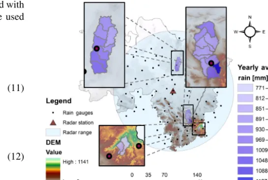
[image:6.612.271.544.67.250.2]The transparent blue circle in Fig. 1 with a 128 km ra-dius is the area being scanned by the Hanover weather radar, whereas the points represent the 53 rain gauges considered in this study. The digital elevation model shows that the north-ern part of the study area is relatively flat and a region with mountainous characteristics is in the southeastern part. The precipitation amount also varies within the study area from around 500 mm yr−1 in the north to 1700 mm yr−1 in the mountains (Berndt et al., 2014). The mean annual rainfall in Fig. 1 for each subcatchment shows also the spatial rainfall variation over the study area. Those values are derived from radar data from 2006 to 2010. This is more evident for the
Figure 1.Study area, catchments, station network and mean annual precipitation (MAP) from 2006 to 2010 from radar data. From north to south: Böhme, Nette and Sieber catchments.
Nette catchment as the southeastern subcatchment receives a larger amount of rainfall than the other subcatchments. Al-though the Sieber catchment is located in the mountainous area, the mean annual rainfall is relatively low. This could be explained by the fact that the catchment is located at the leeward side of the mountains considering the usual west-to-east weather front moving direction.
3.1 Catchments
Three catchments of the Aller–Leine River basin, which have different characteristics, are considered in this study, Fig. 1. Not only are the characteristics of the catchments important but also the locations of the rain gauges. The Böhme catch-ment located in the northern part (with a relatively flat ter-rain) contains eight subcatchments and covers 285 km2. This catchment varies between 50 and 150 m in elevation and con-tains one rainfall station. The Nette catchment has 10 sub-catchments covering 309 km2 and is partly located in the mountainous area, where the elevation reaches up to 550 m. In contrast, the northern part of this catchment is mostly flat. An important point worth mentioning here is that the only station available in this catchment is located in front of the hillside in the southern part. The Sieber catchment is located completely in the mountainous area and has two subcatch-ments covering 45 km2. There are some stations close to the catchment, but no stations are available within it.
3.2 Radar rainfall
dx-Figure 2.XanonexW–Rrelationship (Rabiei et al., 2013).
radar product provided by the DWD is used and processed as following. First, the reflectivity (Z in mm6m−3) is trans-formed to rain intensity (R in mm h−1) by the following re-lationship:
Z=a·Rb. (14)
Standard DWD parameters (Riedl, 1986; Seltmann, 1997) are used, where a=256 and b=1.42. A straightforward clutter detection similar to that of Berndt et al. (2014) is applied thereafter. The final step is to interpolate the rain intensities on rectangular grids using the inverse dis-tance weighted (IDW) technique. This produces rainfall of 1 km×1 km spatial resolution. Afterwards, the mean field bias method (see Sect. 2.1) is implemented to adjust radar data with the observed rain gauge data.
As the observed data are not used directly for the objec-tives of this study, it is decided not to describe them here to avoid any confusion.
3.3 W–Rrelationship
Rabiei et al. (2013) used a linear regression model to describe theW–Rrelationship between the Xanonex sensor readings and rain intensity. Figure 2 illustrates this linear relationship witha=0.2408 andb= −5.4915 (Eq. 4). The dots repre-sent the observations in the laboratory, whereas the dashed lines show the 95 % prediction limits. A detailed descrip-tion of the laboratory experiments is provided in Rabiei et al. (2013). The main disadvantage is when facing small rain-fall values. As mentioned, by considering this relationship and the error distribution for linear regression, negative rain rates can be estimated.
4 Results and discussion
[image:7.612.308.549.64.222.2]In the following, the results of the steps taken for investigat-ing the benefit of usinvestigat-ing RCs for areal rainfall estimation as well as discharge simulation are presented and discussed.
[image:7.612.97.244.66.207.2]Figure 3.The road network on which the RCs are modeled.
Table 1.Number of cars driving at the same time for each RC sce-nario in each catchment.
5 % 4 % 3 % 2 % 1 %
Böhme 38 30 23 15 8
Nette 138 110 83 55 28
Sieber 14 11 8 6 3
4.1 Traffic model
The number of cars is estimated using Eq. (2). It is assumed that only a small portion of cars is equipped with sensors measuring rainfall. In this study, from 1 to 5 % of all cars on the roads are considered to measure rainfall which describes all the RC scenarios. For each 5 min time step, the number of cars is calculated for the 5 % scenario. The other scenar-ios are generated therefrom. Table 1 depicts different RCs’ scenarios considered in this study.
Figure 3 shows the road network considered for the three catchments. As seen in Table 1, a denser network than for the other catchments is available for the Nette catchment. As the Nette catchment is partly located in mountainous area, even this denser network might not provide enough information. This is due to the fact that the RCs are not available overall because of the road network. For that reason, in subcatch-ments such as the southeastern subcatchment, the number of available RCs is lower than in the other subcatchments. 4.2 Network density
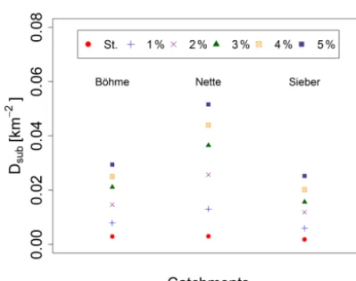
Before illustrating the results of the simulations, i.e., areal rainfall as well as runoff simulation comparison, the network densities using Eq. (3) for different scenarios are presented. This helps to determine whether the network density influ-ences the results.
[image:7.612.345.512.288.342.2]Figure 4.Network density of the catchments for different scenarios.
scenarios have a higher density than the rain gauge network. Depending on the accuracy of the measurement devices, i.e., RCs or rain gauges, the network density has a variable influ-ence. A more detailed investigation is provided in Sect. 4.6.2. 4.3 RainCars uncertainty
The uncertainty related to rainfall estimation by RCs is de-scribed by Eqs. (4) to (6), where ε represents the random error. The normal distribution that defines the random error for each signal reading (signal length) corresponding to each rain rate has the residual variance estimated by the vertical distances between the observations and the regression line. The random error, log(ε), is then simulated using the normal distribution. As discussed earlier, a power regression model describes theW–Rrelationship in this study.
Figure 5a shows theW–Rrelationship after log–log trans-formation. The same assumption as before is valid, namely that the random error is normally distributed and derived from the deviation between observation points and the lin-ear regression model. Figure 5b illustrates theW–R relation-ship implemented in this study. It is derived using the fol-lowing steps: (1) applying log–log transformation on both axes, (2) applying linear regression on the transformed data (Fig. 5a), (3) estimating the residual variance for the normal distribution describing the random error for the linear regres-sion model and (4) transferring the data back for practical use (Fig. 5b). The coefficient of determination given in Fig. 5b is estimated using the transformed log–log regression model in Fig. 5a.
The data transformation has, in general, two important ef-fects on theW–Rrelationship: (1) preventing the derivation of unrealistic rain rates and (2) skewing the distribution of random error. The latter aspect affects also the prediction limit in Fig. 5. As can be seen in Fig. 5b, the upper and lower limits bend when they are further from the origin, which re-sults in larger inaccuracy for the rain rate estimated by RCs for higher rainfall intensities. On the other hand, the positive
skewness introduces a positive bias that causes overestima-tion when estimating rain rate by RCs. This can be seen when comparing the distances from the model line to the upper and lower prediction limits. Although theW–R relationship has this deficiency, a larger number of RCs and more accurate optical sensors can help compensate this problem. These two aspects are addressed in Sect. 4.6.2. and 4.6.3, respectively.
4.4 Variogram properties used in this study
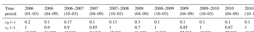
The properties of the variograms used in this study are pro-vided in Table 2.
The variograms are fitted using radar data in 11 differ-ent (mostly 6-month intervals) over the 5 years with 5 min temporal resolution. The goal is to interpolate rain gauges as well as rainfall from RCs on a 5 min temporal resolution. A large relative range is estimated in wintertime, which il-lustrates different seasonal rainfall patterns. It supports the seasonal separation for interpolating the data which were discussed earlier. As can be seen, the properties of the var-iograms change even among the same seasons in different years. Therefore, it was decided to use the variable vari-ograms provided in Table 2. It was mentioned earlier that negative estimated values were set to zero. However, the nugget values provided in Table 2 illustrate the low possi-bility of facing negative estimation values.
4.5 Reference discharge
As mentioned earlier, the simulated discharge for different scenarios will be compared with the reference discharge. The reference discharge, the benchmark, is simulated using radar data after applying mean field bias correction (creating the reference rainfall data) as input to the HBV-IWW model us-ing pre-calibrated model parameters. Because of the lumped approach for calibrating the model parameters and the sub-catchments with relatively small size, the rainfall characteris-tics, especially the spatial pattern, are the highest influencing factors in discharge simulation.
The performance of the HBV-IWW model is evaluated on an hourly temporal resolution. Therefore, an aggregation of 5 min interpolation data to hourly data is carried out before using it in the hydrological model.
4.6 Comparing areal rainfall and simulated discharge for different sources
Figure 5. (a)Xanonex log-transformedW–Rrelationship after Eq. (6).(b)XanonexW–Rrelationship after Eq. (5); the red lines illustrate the 95 % prediction limits.
Table 2.Theoretical variogram model parameters used in this study;aeffis the effective rangeccthe sill andc0the nugget effect.
Time 2006 2006 2006–2007 2007 2007–2008 2008 2008–2009 2009 2009–2010 2010 2010
period (01–03) (04–09) (10–03) (04–09) (10–03) (04–09) (10–03) (04–09) (10–03) (04–09) (10–12)
c0(–) 0.2 0.1 0.17 0.1 0.13 0.3 0.1 0.1 0.1 0.1 0.1
cc(–) 1 0.9 0.9 0.85 1 0.7 1 0.85 1 0.87 1
aeff(m) 60 000 24 000 42 000 24 000 42 000 36 000 48 000 22 500 45 000 27 000 48 000
4.6.1 Rain gauge network Areal rainfall estimation
The areal rainfall estimations corresponding to the three catchments shown in Fig. 1 are compared with the reference data. It should be noticed again that the comparison is carried out after interpolating the data with 5 min temporal resolu-tion and aggregating the data to hourly temporal resoluresolu-tion because of the required temporal resolution for the hydro-logical model.
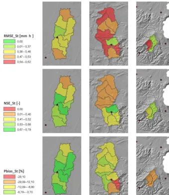
Figure 6 provides the statistical measures for the three catchments under investigation when evaluating the quality of areal rainfall estimation using only rain gauges. This is carried out by comparing the estimated areal rainfall using rain gauges and implementing OK with the reference data.
For the Böhme catchment, having one station in the catch-ment and one close by provides sufficient rainfall informa-tion. As expected, the closer the subcatchments to the sta-tions, the better the quality of areal rainfall estimation. The areal rainfall estimated for the northernmost subcatchment is not as good as for the other subcatchments because there is no station nearby. Although the potential for improving RMSE and NSE values exists, the Pbias criterion is in gen-eral relatively low. This means that the total water volume is estimated relatively well, and therefore for purposes such as hydrological modeling the quality of areal rainfall estimation might be sufficient. In all cases, polygons with green color represent better results than the red ones.
The Nette catchment, the subcatchment that includes a sta-tion, as expected, has a superior rainfall estimation quality to the other subcatchments. Unpredictably, the quality of areal rainfall estimation for the other subcatchments close to the station is weak. For example, although the two southern sub-catchments are in the vicinity of a station, the statistical mea-sures are relatively poor. A rapid change in elevation is ev-ident when considering the DEM map in Fig. 1. Assuming that rainfall characteristics change along the elevation gradi-ent, a change in the spatial rainfall pattern is expected. The single station is no longer able to provide the actual rainfall even for the surrounding subcatchments. This is in contrast to the Böhme catchment where the DEM map shows a flat catchment and the only station on the Böhme catchment is sufficient for areal rainfall estimation.
Although the Sieber catchment is smaller than the other two catchments and is expected to be more easily modeled, the catchment is located in a mountainous region and suffers from the fact that no rain gauge is available directly within the catchment. Due to these facts, the areal rainfall estimation is rather poor, especially when the Pbias is of concern. For such conditions, additional means of rainfall measurement would be beneficial.
Discharge simulation
[image:9.612.55.537.291.352.2]Figure 6.Areal rainfall estimation using rain gauges compared with the reference data in, from left to right, the Böhme, Nette and Sieber catchments. Locations of the rain gauges are marked by black dots. The polygons near the green color present better results than the ones near the red color.
Table 3.Simulated discharge by rain gauges compared with the ref-erence data.
Böhme Nette Sieber
RMSE (m3s−1) 0.98 2.8 0.51
NSE (–) 0.95 0.76 0.86
Pbias (%) −6.2 −22.5 −15.8
pattern, each catchment responds differently when only rain gauges are used. The reference discharge, the benchmark, is simulated using reference areal rainfall, i.e., radar data after MFB, and the pre-calibrated model parameters.
Table 3 provides the statistical measures of simulated dis-charges when only rain gauges are implemented. Although both the Böhme and Nette catchments benefit from having
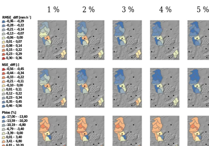
[image:10.612.75.257.549.606.2]Figure 7.Areal rainfall estimation evaluation using RCs for the Böhme catchment. The blue color for RMSEdiffand NSEdiffillustrates the improvement of the areal rainfall estimation quality when RCs are used compared with when only rain gauges are considered.
-0,36 – -0,29 -0,28 – -0,22 -0,21 – -0,14 -0,13 – -0,07 -0,06 – 0,00 0,01 – 0,07 0,08 – 0,14 0,15 – 0,22 0,23 – 0,29 0,30 – 0,36
NSE_diff [-] -0,56 – -0,45 -0,44 – -0,34 -0,33 – -0,22 -0,21 – -0,11 -0,10 – 0,00 0,01 – 0,11 0,12 – 0,22 0,23 – 0,34 0,35 – 0,45 0,46 – 0,56
Pbias [%] -17,00 – -13,60 -13,59 – -10,20 -10,19 – -6,80 -6,79 – -3,40 -3,39 – 0,00 0,01 – 3,40 3,41 – 6,80 6,81 – 10,20 10,21 – 13,60 13,61 – 17,00 -1 RMSE_diff [mm h ]
1 % 2 % 3 % 4 % 5 %
Figure 8.Areal rainfall estimation evaluation using RCs for the Nette and Sieber catchment. The blue color for RMSEdiff and NSEdiff illustrates the improvement of the areal rainfall estimation quality when RCs are used compared with when only rain gauges are considered.
be sufficient for areal rainfall estimation for a flat catchment such as the Böhme catchment and would not be sufficient for a catchment such as the Nette catchment, which is partly located in the mountainous area. There is no station located in the Sieber catchment, which explains the poor Pbias in Table 3, although the other two criteria are rather good. In
[image:11.612.131.467.357.593.2]4.6.2 RCs against rain gauges using errors from laboratory experiments
Areal rainfall estimation
A similar strategy is pursued for the moving cars measuring rainfall. As before, the evaluation involves two parts. First, the areal rainfall estimation by implementing RCs is com-pared with the reference rainfall. Thereafter, the simulated discharges are compared after using the data in the HBV-IWW hydrological model.
The benefit of using RCs for areal rainfall estimation can be assessed when their performance is compared with the standard approach, i.e., using only the rain gauges. To this end, after estimating the statistical measures by comparing with reference data, the difference between the statistical measures is addressed. This means that, for example, for the root mean square error RMSEdiff=RMSERCs −RMSESt.
As a result, negative RMSEdiff values as well as positive
NSEdiffvalues represent better areal rainfall estimation when
using RCs compared to stations. For Pbias, the specific val-ues are compared without building differences.
Figure 7 illustrates the statistical measures for the Böhme catchment when the RCs are used for areal rainfall estima-tion. Implementing RCs in general results in better areal rain-fall estimation. As expected, the improvement in subcatch-ments away from the stations is more significant than the ones close to them. Also, the number of cars plays an im-portant role. If the number of RCs increases, the quality of areal rainfall estimation improves. Considering only the two mentioned criteria, using RCs for areal rainfall estimation is always superior to using stations in this catchment. The im-provement for each subcatchment varies depending on the number of RCs as well as the location of the station. PbiasRCs
values show an overestimation of areal rainfall because of the positive skew of the error distribution as explained ear-lier (see Fig. 5b).
Figure 8 illustrates the statistical measures for different RC scenarios in the Nette and Sieber catchments.
The use of RCs for rainfall estimation in the Nette catch-ment has similar advantages as for the Böhme catchcatch-ment. In contrast to that, RCs are not always beneficiary in the Nette catchment. A detailed investigation shows that the rainfall es-timation for the subcatchment in which the station is located is hard to beat by using RCs. In contrast to all the subcatch-ments where an overestimation is observed, for the Nette basin, the subcatchment with red color in Pbias responds dif-ferently. This can be explained by the RC network density. This part of the catchment suffers from the fact that RCs are rarely available because there are fewer roads, as it is located in the mountainous part.
For the Sieber catchment, using RCs also results in better areal rainfall estimation. Increasing the number of RCs has again advantages. The improvement in areal rainfall estima-tion is not as strong as in the other catchments because of the
existing stations in the vicinity of the catchment. Although RMSE and NSE do not vary significantly, comparing with Fig. 6, the Pbias criterion improves meaningfully.
It should be noted that although the Nette catchment bene-fits from a denser RC network (Fig. 4), because of the spatial rainfall pattern, the need for a higher number of RCs or a better location for the only station is evident.
4.6.3 Discharge simulation
Table 4 provides the statistical measures of simulated dis-charges when RCs are implemented. The first column, titled “St.”, refers to when only rain gauges are considered, which is included here again to facilitate easy comparison.
Although the Böhme catchment performs the best among the three catchments when only rain gauges are considered, using RCs is still useful. Figure 8 shows that the areal rain-fall estimation improves slightly when using RCs. For anal-yses requiring fine temporal and spatial resolution data, e.g., urban hydrology, using RCs may improve the simulation re-sults more evidently. Due to the fact that the improvement in discharge simulation is not very strong in this catchment, with the given temporal and spatial resolution, for such stud-ies the need for using RCs can be considered inessential.
As discussed earlier, because of the characteristics of the Nette catchment, this catchment has the highest potential for improvement by RCs. Implementing even a small number of RCs improves the results significantly. As seen in Fig. 4, the Nette catchment has the highest RC network density among the three catchments. This explains the better performance in this catchment. As expected, positive Pbias in the simulated discharge indicates overestimation, which follows the areal rainfall overestimation observed earlier.
Unlike the other catchments, the Sieber catchment is lo-cated in the mountainous area. The NSE and RMSE crite-ria do not improve significantly when using RCs. Taking a deeper look at the traffic model data, from 1 % scenario to 5 % scenario, the number of cars measuring rainfall is 3, 6, 8, 11 and 14, respectively (see Table 1). Only two scenarios can result in better discharge simulation (4 and 5 %) indicat-ing the least required RC network density for this catchment. As with the other two catchments, using RCs results in the overestimation of the discharge.
Addi-Table 4.Simulated discharge by RCs compared with the reference data.
Catchment St. 1 % RCs 2 % RCs 3 % RCs 4 % RCs 5 % RCs
RMSE (m3s−1) 0.98 0.66 0.6 0.61 0.6 0.57
Böhme NSE (–) 0.95 0.98 0.98 0.98 0.98 0.98
Pbias (%) −6.2 6.4 6.1 7.4 7.6 7.4
RMSE (m3s−1) 2.8 1.01 0.84 0.67 0.73 0.76
Nette NSE (–) 0.76 0.97 0.98 0.99 0.98 0.98
Pbias −22.5 4.8 6.8 5 6.7 7.2
RMSE (m3s−1) 0.51 0.55 0.58 0.53 0.48 0.37
Sieber NSE (–) 0.86 0.83 0.81 0.84 0.88 0.92
[image:13.612.111.485.85.222.2]Pbias (%) −15.8 7.5 6 4.7 3.2 2.6
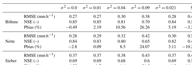
Table 5.Uncertainties for RCs when estimating areal rainfall and averaging over all subcatchments; the 5 % traffic model is considered.
σ2=0.0 σ2=0.01 σ2=0.04 σ2=0.09 σ2=0.021 St.
RMSE (mm h−1) 0.27 0.27 0.30 0.38 0.28 0.44
Böhme NSE (–) 0.85 0.85 0.81 0.70 0.84 0.58
Pbias (%) −0.49 2.19 10.56 26.26 5.19 −3.22
RMSE (mm h−1) 0.28 0.29 0.32 0.42 0.30 0.53
Nette NSE (–) 0.84 0.83 0.80 0.65 0.82 0.43
Pbias (%) −2.8 0.09 8.5 24.07 3.11 −10.21
RMSE (mm h−1) 0.37 0.37 0.38 0.43 0.37 0.46
Sieber NSE (–) 0.69 0.69 0.68 0.6 0.69 0.53
Pbias (%) −4.55 −1.7 6.4 21.5 1.2 −14.45
tionally, even a small number of RCs can improve the dis-charge simulation significantly. Depending on the quality of the required hydrological analyses, the need for the use of RCs is open to discussion. Basically, a higher number of equipped cars are needed for mountainous catchments in this study area than for flat catchments. In other words, the need for increasing the number of observations is evident when the spatiotemporal variation of rainfall is high.
4.6.4 RCs against rain gauges using hypothetical errors Areal rainfall estimation
The minimum rainfall measurement accuracy required for the RCs to be useful is investigated in this section. All the different accuracies are addressed for the 5 % RC scenario specifically. The error for the linear model is estimated on the log–log transformed data (Fig. 5). The normal distribution was defined by the variance (σ2), equal to 0.021, from lab-oratory experiment results. In order to investigate the impor-tance of the error on the results, four other variances of 0.0, 0.01, 0.04 and 0.09 are considered. At the end, the areal rain-fall estimation quality as well as the performance of the hy-drological model was compared with that of using the orig-inal variance from the laboratory. Table 5 provides the
aver-aged statistical measures for each catchment. The areal rain-fall estimation considering different errors for RCs is com-pared with the reference data. The same assumptions as ear-lier (see Sect. 4.3) are taken with different variances for the distribution function representing the error range. St. repre-sents the areal rainfall estimation performance when only the rain gauges are implemented.
The rainfall overestimation by implementing higher σ2 values is evident. For all catchments even assuming a rela-tively large uncertainty ofσ2=0.09, NSE and RMSE values improve compared with when only rain gauges are consid-ered. As the Pbias is quite large forσ2=0.04 andσ2=0.09, the use of RCs for areal rainfall estimation is questionable. In fact, for such cases, using rainfall data observed by RCs could be considered as additional information for areal rain-fall estimation, e.g., Kriging with external drift or Kriging with uncertain data.
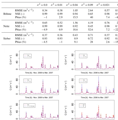
[image:13.612.97.497.259.395.2]Table 6.Investigating different uncertainties for RCs when simulating discharge compared with the reference discharge; the 5 % traffic model is considered.
σ2=0.0 σ2=0.01 σ2=0.04 σ2=0.09 σ2=0.021 St.
RMSE (m3s−1) 0.34 0.38 1.05 2.64 0.57 0.98
Böhme NSE (–) 0.99 0.99 0.94 0.65 0.98 0.95
Pbias (%) −1 2.9 15.5 40 7.4 −6.2
RMSE (m3s−1) 0.65 0.52 1.56 4.19 0.76 2.8
Nette NSE (–) 0.99 0.99 0.92 0.45 0.98 0.76
Pbias (%) −4.9 0.9 18.6 52.6 7.2 −22.5
RMSE (m3s−1) 0.37 0.36 0.43 0.71 0.37 0.51
Sieber NSE (–) 0.93 0.93 0.9 0.72 0.92 0.86
Pbias (%) −4.5 −1 9.1 28 2.6 −15.8
Ref σ = 0.0
Ref σ = 0.2
Ref σ = 0.145 (lab)
Ref σ = 0.1
Ref σ = 0.3
Ref St.
Q [m
3 s -1]
Q [m
3 s -1]
Q [m
3 s -1]
Q [m
3 s -1]
Q [m
3 s -1]
Q [m
3 s -1]
Figure 9.Discharge simulation using different sources of data for the Nette catchment between November 2007 and March 2008. For RCs, only the 5 % scenario is considered.
and maxima over the study area can lead to overestimation and underestimation, respectively. It is more probable to miss maxima than minima due to the fact that high rainfall inten-sities may occur in places where no RCs or rain gauge ob-servations are available. Minima can be captured easier than maxima as it covers a larger area, illustrating the positive skewness of the rain rate distribution. This might explain the minor negative Pbias derived by RCs even whenσ=0.0.
4.6.5 Discharge simulation
Table 6 provides the averaged statistical measures of the sim-ulated discharges for each catchment when the 5 % RC sce-nario is considered. As expected, the best performance be-longs to the RCs scenario for which the measurement error
imple-menting quantile mapping like the one introduced by Rabiei and Haberlandt (2015).
As observed, the improvement of model performance in the Nette catchment when using RCs is more evident than for the other two catchments. Therefore, it is decided to in-vestigate the Nette catchment in more detail by analyzing the hydrographs for all the scenarios given in Table 6.
Figure 9 shows the simulated discharge between Novem-ber 2006 and March 2007. It can be observed that when only rain gauges (St.) are used, the model misses some peaks and performs poorly. This illustrates that the local rainfall is often not captured. The model performance improves significantly when using RCs. By increasing the uncertainties, i.e., enlarg-ingσ2, the overestimation of rainfall affects the model per-formance as well. Considering the uncertainties larger than the uncertainty derived from laboratory experiments could in fact illustrate situations that we may encounter in practice and we did not consider here.
5 Summary and conclusion
The value of using moving cars for rainfall measurement pur-poses (RCs) was investigated with laboratory experiments by Rabiei et al. (2013). They analyzed the Hydreon and Xanonex optical sensors against different rainfall intensities. The optical sensors showed promising results when used for point rainfall measurement. Because of the low number of real RCs available on roads, the main objective of this study was to implement and investigate the errors derived from the laboratory experiments for areal rainfall estimation in a com-puter simulation. The errors were considered for the theoret-ical RCs, provided by a traffic model, and OK was imple-mented for areal rainfall estimation. Thereafter, the data are also used for discharge simulations in the HBV hydrological model. The value of the RCs is compared with when only rain gauges are implemented. Radar data were considered as the reference data to directly evaluate the areal rainfall esti-mation rather than following the common approach for eval-uating an interpolation technique, i.e., cross validation. The other sources of data, i.e., RCs and rain gauges, were ex-tracted from the reference data source, accordingly. A period of 5 years from 2006 to 2010 and three catchments with dif-ferent characteristics are considered.
The results of the study are as follows:
1. Implementing RCs with the uncertainties derived from the laboratory experiments improves the quality of mod-eled areal rainfall estimation compared with when only rain gauges are used. The same is valid for discharge simulation when the estimated areal rainfall is imple-mented in hydrological modeling. However, the im-provement is observed to be strongly dependent on the catchment characteristics, RC network density and spa-tial variability of rainfall.
2. Because of the positive bias of the error distribution when using a log-transformedW–R relationship, areal rainfall overestimation is observed, in general, which re-sulted in an overestimation of discharges as well. This can be compensated by either increasing the RC net-work density or implementing more accurate optical sensors.
3. By increasing the rainfall measurement uncertainty by RCs, i.e., assuming larger variances for the random er-ror, rainfall overestimation increases significantly. Im-plementing errors up to a certain level is worthwhile, whereas larger uncertainties resulted in deterioration of results. Although the RCs with large errors should not be considered directly for rainfall measurement, rela-tively good NSE values show the potential of RCs to be regarded as additional information in interpolation tech-niques.
4. It is observed that applying OK for the interpolation of point values for areal rainfall estimation results in derestimation of rainfall. This was seen when no un-certainty was considered for RCs as well as for the case when only rain gauges were involved. The non-Gaussianity of data and missing the rainfall maxima by ground observations (RCs or rain gauges) over the study area may explain this phenomenon.
The hydrological simulations are carried out on hourly tem-poral resolution data with a lumped model parameter ap-proach where the areal rainfall for each subcatchment is es-timated separately. The conclusion of this study may not be valid for other cases when, for example, a distributed model or a different temporal resolution is being investigated. De-pending on the target of each study, higher levels of data quality may be required. For instance, following the conclu-sions by Schilling (1991), in which he discussed implement-ing high spatial (1 km2) and temporal (1 min) resolution data for urban hydrology, the quality of rainfall measurement by RCs might be insufficient. Furthermore, Berne et al. (2004) also concluded that a temporal resolution of about 5 min and a spatial resolution of about 3 km are required for ur-ban catchments with an area about 1000 ha. They also stated that for smaller catchments with an area about 100 ha, higher resolution of about 3 min and 2 km are needed.
Acknowledgements. The study was funded by the German Re-search Foundation (DFG, 3504/5-2). The authors thank the German Weather Service (DWD) for the meteorological data. Moreover, the authors wish to thank Anne Fangmann and Sarah Louise Collins for their comments on an earlier draft of the paper. The authors are very thankful to the associated editor, G. Pegram and one anonymous referee for their critical remarks on the manuscript to improve the paper.
The publication of this article was funded by the open-access fund of Leibniz Universität Hannover.
Edited by: R. Uijlenhoet
Reviewed by: G. Pegram and one anonymous referee
References
Berndt, C., Rabiei, E., and Haberlandt, U.: Geostatistical merging of rain gauge and radar data for high temporal resolutions and various station density scenarios, J. Hydrol., 508, 88–101, 2014. Berne, A., Delrieu, G., Creutin, J.-D., and Obled, C.: Temporal and spatial resolution of rainfall measurements required for urban hy-drology, J. Hydrol., 299, 166–179, 2004.
de Jong, S.: Low cost disdrometer, master thesis report, TU Delft, 2010.
Haberlandt, U. and Sester, M.: Areal rainfall estimation using mov-ing cars as rain gauges – a modellmov-ing study, Hydrol. Earth Syst. Sci., 14, 1139–1151, doi:10.5194/hess-14-1139-2010, 2010. Hydreon: Rain Gauge Model RG-11 Instructions, available at: http:
//www.rainsensors.com/ (last access: 19 September 2016), 2015. Isaaks, E. H. and Srivastava, R. M.: An Introduction to Applied
Geostatistics, Oxford Univ. Press, New York, 278–322, 1990. Kidd, C. and Huffman, G.: Global precipitation measurement,
Me-teorol. Appl., 18, 334–353, 2011.
Kidd, C. and Levizzani, V.: Status of satellite precipita-tion retrievals, Hydrol. Earth Syst. Sci., 15, 1109–1116, doi:10.5194/hess-15-1109-2011, 2011.
Kirkpatrick, S.: Optimization by simulated annealing: Quantitative studies, J. Stat. Phys., 34, 975–986, 1984.
Lindström, G., Johansson, B., Persson, M., Gardelin, M., and Bergström, S.: Development and test of the distributed HBV-96 hydrological model, J. Hydrol., 201, 272–288, 1997.
Nash, J. E. and Sutcliffe, J. V.: River flow forecasting through con-ceptual models part I – A discussion of principles, J. Hydrol., 10, 282–290, 1970.
Overeem, A., Leijnse, H., and Uijlenhoet R.: Country-wide rainfall maps from cellular communication networks, P. Natl. Acad. Sci., 11, 2741–2745, 2013.
Prakash, S., Mitra, A. K., Pai, D. S., and AghaKouchak, A.: From TRMM to GPM: How well can heavy rainfall be detected from space?, Adv. Water Resour., 88, 1–7, 2016.
Rabiei, E. and Haberlandt, U.: Applying bias correction for merging rain gauge and radar data, J. Hydrol., 522, 544–557, 2015. Rabiei, E., Haberlandt, U., Sester, M., and Fitzner, D.:
Rain-fall estimation using moving cars as rain gauges – labora-tory experiments, Hydrol. Earth Syst. Sci., 17, 4701–4712, doi:10.5194/hess-17-4701-2013, 2013.
Rahimi, A. R., Holt, A. R., Upton, G. J. G., Krämer, S., Redder, A., and Verworn, H. R.: Attenuation Calibration of an X-Band Weather Radar Using a Microwave Link, J. Atmos. Ocean. Tech-nol., 23, 395–405, 2006.
Riedl, J.: Radar-Flächenniederschlagsmessung, Promet, 20–23, 1986.
Schilling, W.: Rainfall data for urban hydrology: what do we need?, Atmos. Res., 27, 5–21, 1991.
Seltmann, J.: Radarforschung im DWD: Vom Scan zum Produkt, Promet, 32–42, 1997.
Shrestha, R., Tachikawa, Y., and Takara, K.: Input data resolution analysis for distributed hydrological modeling, J. Hydrol., 319, 36–50, 2006.
Silverman, B. W.: Density Estimation for Statistics and Data Anal-ysis, 26, RC Press, 1986.
Upton, G. J. G., Holt, A. R., Cummings, R. J., Rahimi, A. R., and Goddard, J. W. F.: Microwave links: The future for urban rainfall measurement?, Atmos. Res., 77, 300–312, 2005.
Wallner, M. and Haberlandt, U.: Non-stationary hydrological model parameters: a framework based on SOM-B, Hydrol. Process., 29, 3145–3161, 2015.
Xanonex: Xanonex Funktionsweise, available at: http://www. xanonex.de/ (last access: 19 September 2016), 2015.
Xu, H., Xu, C.-Y., Chen, H., Zhang, Z., and Li, L.: Assessing the influence of rain gauge density and distribution on hydrological model performance in a humid region of China, J. Hydrol., 505, 1–12, 2013.