Physics and Astronomy Dissertations Department of Physics and Astronomy
Spring 5-7-2011
The Self-Calibration Method for Multiple Systems at the CHARA
The Self-Calibration Method for Multiple Systems at the CHARA
Array
Array
David P. O'Brien
Georgia State University
Follow this and additional works at: https://scholarworks.gsu.edu/phy_astr_diss
Part of the Astrophysics and Astronomy Commons, and the Physics Commons
Recommended Citation Recommended Citation
O'Brien, David P., "The Self-Calibration Method for Multiple Systems at the CHARA Array." Dissertation, Georgia State University, 2011.
https://scholarworks.gsu.edu/phy_astr_diss/48
This Dissertation is brought to you for free and open access by the Department of Physics and Astronomy at ScholarWorks @ Georgia State University. It has been accepted for inclusion in Physics and Astronomy
Dissertations by an authorized administrator of ScholarWorks @ Georgia State University. For more information,
THE SELF-CALIBRATION METHOD FOR MULTIPLE SYSTEMS AT THE
CHARA ARRAY
by
DAVID O’BRIEN
Under the Direction of Harold A. McAlister
ABSTRACT
The self-calibration method, a new interferometric technique using measurements in
theK′
-band (2.1µm) at the CHARA Array, has been used to derive orbits for several
spectroscopic binaries. This method uses the wide component of a hierarchical triple
system to calibrate visibility measurements of the triple’s close binary system through
quasi-simultaneous observations of the separated fringe packets of both. Prior to the
onset of this project, the reduction of separated fringe packet data had never included
the goal of deriving visibilities for both fringe packets, so new data reduction software
has been written. Visibilities obtained with separated fringe packet data for the target
close binary are run through both Monte Carlo simulations and grid search programs
in order to determine the best-fit orbital elements of the close binary.
Several targets, with spectral types ranging from O to G and luminosity classes
from III to V, have been observed in this fashion, and orbits have been derived for the
for the calculation of the masses of the components in these systems. The magnitude
differences between the components can also be derived, provided that the
compo-nents of the close binary have a magnitude difference of ∆K <2.5 (CHARA’s limit).
Derivation of the orbit also allows for the calculation of the mutual inclination (Φ),
which is the angle between the planes of the wide and close orbits. According to data
from the Multiple Star Catalog, there are 34 triple systems other than the 8 studied
here for which the wide and close systems both have visual orbits. Early formation
scenarios for multiple systems predict coplanarity (Φ < 15◦), but only 6 of these 42
systems are possibly coplanar. This tendency against coplanarity may suggest that
the capture method of multiple system formation is more important than previously
believed.
THE SELF-CALIBRATION METHOD FOR MULTIPLE SYSTEMS AT THE
CHARA ARRAY
by
DAVID O’BRIEN
A Dissertation Presented in Partial Fulfillment of Requirements for the Degree of
Doctor of Philosophy
in the College of Arts and Sciences
Georgia State University
THE SELF-CALIBRATION METHOD FOR MULTIPLE SYSTEMS AT THE
CHARA ARRAY
by
DAVID O’BRIEN
Major Professor:
Committee:
Harold A. McAlister
Nikolaus Dietz
Douglas Gies
Todd Henry
Russel White
Electronic Version Approved:
Office of Graduate Studies
College of Arts & Sciences
Georgia State University
Dedication
v
– 0 –
Acknowledgments
I would like to thank my family for their constant support and trust, without which
this dissertation would not have been possible. Special thanks to my adviser, Dr.
Harold McAlister, for guiding me through several difficult years of working on this
project. To Dr. Douglas Gies and Dr. Theo ten Brummelaar, thank you for all
the tips and suggestions as to how to improve this project. To the other CHARA
graduate students, especially Dr. Deepak Raghavan and Dr. Tabetha Boyajian,
thanks for helping me learn how to observe with CHARA and work with CHARA
data. To the other members of my committee, thank you for giving me tips on how to
improve the quality of my document and taking the time out of your busy schedules
to make sure that I am worthy of this honor. Thanks to Rajesh Deo and Justin
Cantrell for helping me out with my numerous computer problems over the years.
Thanks to Saida Caballero-Nieves and Stephen Williams for always helping me out
with coding and formatting and various other issues I have run into. Finally, to Misty
Table of Contents
Acknowledgments . . . v
Tables . . . ix
Figures . . . xii
Abbreviations and Acronyms . . . xvi
1 Introduction . . . 1
1.1 Basic Interferometry . . . 7
1.2 The CHARA Array . . . 14
2 Target List . . . 17
2.1 Observing Criteria . . . 17
2.1.1 The Fourth Catalog of Interferometric Measurements of Binary Stars . . . 20
2.1.2 The 9th Catalogue of Spectroscopic Binary Orbits . . . 21
2.1.3 The Multiple Star Catalog . . . 21
2.2 Observation Planning . . . 26
3 Data Reduction . . . 37
3.1 Initial data processing . . . 37
3.2 Finding separated fringe packets . . . 45
3.3 Fringe fitting . . . 51
3.4 Identifying the fringe packets . . . 55
3.5 Calibration . . . 59
4 Side-Lobe Interference . . . 61
vii
4.2 Simultaneous fitting . . . 73
4.3 Sinusoid fitting of visibility ratio . . . 77
4.4 Adopted correction method . . . 82
5 Results . . . 83
5.1 Orbit fitting procedure . . . 83
5.2 Orbits . . . 88
5.2.1 V819 Her (HD 157482) . . . 88
5.2.2 κ Peg (HD 206901) . . . 106
5.2.3 η Virginis (HD 107259) . . . 119
5.2.4 η Orionis (HD 35411) . . . 128
5.2.5 55 UMa (HD 98353) . . . 139
5.2.6 13 Ceti (HD 3196) . . . 147
5.2.7 CHARA 96 (HD 193322) . . . 155
5.2.8 HD 129132 . . . 166
5.3 Other targets . . . 176
6 Discussion . . . 179
6.1 Mutual Inclination . . . 179
6.1.1 Formation scenarios . . . 179
6.1.2 Distribution of Φ . . . 183
6.2 Evaluation of the Self-Calibration Method . . . 192
6.3 Future Work . . . 197
References . . . 200
Appendices . . . 204
A Calculations of parameters . . . 205
A.1 Calculating ρ and θ . . . 205
A.3 Normalizing separated fringe packet visibilities . . . 209
A.4 Calculating Φmin . . . 211
B Visibility Curves . . . 213
B.1 V819 Her Revised . . . 214
B.2 κ Peg . . . 216
B.3 η Vir . . . 221
B.4 η Ori . . . 223
B.5 55 UMa . . . 228
B.6 13 Ceti . . . 230
B.7 HD 129132 . . . 233
ix
– 0 –
Tables
2.1 Criteria for Target List . . . 20
2.2 Main Target List . . . 24
2.3 Projected Separation Table (in µm) for HD 3196 on 2010 Dec 1 . . . 27
2.4 Targets that produced separated fringe packets . . . 35
4.1 Original and corrected visibility ratios for HD 35411 on 2008 September 12 . . . 72
4.2 Original and corrected visibilities and ratios from simultaneous fitting for HD 35411 and HD 157482 . . . 77
5.1 V819 Her Data . . . 92
5.2 Orbital Elements for V819 Her B derived from minimum χ2 fit . . . . 93
5.3 V819 Her Data Revised . . . 100
5.4 Revised Orbital Elements for V819 Her B derived from minimum χ2 fit 101 5.5 V819 Her Mutual Inclination . . . 104
5.6 V819 Her Masses . . . 104
5.7 Magnitudes of V819 Her components . . . 104
5.8 κ Peg Data . . . 110
5.9 Orbital Elements for κ Peg B derived from minimum χ2 fit . . . 113
5.10 κ Peg Mutual Inclination . . . 117
5.11 κ Peg Masses . . . 117
5.12 Magnitudes of κ Peg components . . . 117
5.13 η Vir Data . . . 123
5.15 η Vir Mutual Inclination . . . 127
5.16 η Vir Masses . . . 127
5.17 Magnitudes of η Vir components . . . 127
5.18 η Ori Data . . . 130
5.19 Orbital Elements for η Ori Aab derived from minimum χ2 fit . . . 134
5.20 η Ori Mutual Inclination . . . 138
5.21 η Ori Masses . . . 138
5.22 Magnitudes of η Ori components . . . 138
5.23 55 UMa Data . . . 141
5.24 Orbital Elements for 55 UMa A derived from minimum χ2 fit . . . 143
5.25 55 UMa Mutual Inclination . . . 146
5.26 55 UMa Masses . . . 146
5.27 Magnitudes of 55 UMa components . . . 146
5.28 13 Ceti Data . . . 149
5.29 Orbital Elements for 13 Ceti A derived from minimum χ2 fit . . . 151
5.30 13 Ceti Mutual Inclination . . . 154
5.31 13 Ceti Masses . . . 154
5.32 Magnitudes of 13 Ceti components . . . 154
5.33 CHARA 96 Data . . . 158
5.34 Orbital Elements for CHARA 96 . . . 162
5.35 HD 129132 Data . . . 168
5.36 Orbital Elements for HD 129132 Aa derived from minimum χ2 fit . . 171
5.37 HD 129132 Mutual Inclination . . . 175
5.38 HD 129132 Masses . . . 175
xi
5.40 SCAM Queue Observing . . . 178
6.1 All Known Mutual Inclinations . . . 184
6.2 Mutual Inclinations for Selected Close Binaries . . . 192
6.3 Mass Comparison . . . 196
6.4 Future SCAM Targets by HD No. . . 198
Figures
1.1 Young’s Double-Slit Experiment . . . 9
1.2 Polychromatic Fringes . . . 10
1.3 Visibility Dependence on Angular Diameter . . . 11
1.4 Visibility Dependence on Separation . . . 12
1.5 Visibility Dependence on Magnitude Difference . . . 13
1.6 The CHARA Array . . . 14
1.7 CHARA Classic . . . 16
2.1 Separated Fringe Packets at Threshold of Simultaneous Observation . 29 2.2 Coherence Length . . . 30
2.3 Fully Visible Separated Fringe Packets . . . 31
2.4 Side-Lobe Interference . . . 33
2.5 Separated Fringe Packets at Lower Limit of Observation . . . 34
3.1 Typical raw data from a single detector . . . 39
3.2 Dark noise-subtracted data . . . 42
3.3 Normalization . . . 43
3.4 Bandpass filtering . . . 44
3.5 Bandpass-filtered scan . . . 45
3.6 Fringe envelope of a single scan . . . 46
3.7 Shift-and-add envelope . . . 47
3.8 Locating fringe packets . . . 50
xiii
3.10 Identifying fringe packets . . . 58
4.1 Side-Lobe Interference Effect . . . 62
4.2 Side-Lobe Interference Modeling for a Visibility Ratio of 1 . . . 64
4.3 Side-Lobe Interference Modeling for a Visibility Ratio of 1.5 . . . 65
4.4 Side-Lobe Interference Modeling for a Visibility Ratio of 2 . . . 66
4.5 Side-Lobe Interference Modeling for a Visibility Ratio of 3 . . . 67
4.6 Visibility ratio as a function of separation . . . 68
4.7 Visibility ratio as a function of separation (cont’d) . . . 69
4.8 Deconstructing the SSFPs . . . 71
4.9 Example simultaneous fits . . . 75
4.10 Original vs. corrected visibility ratio for simultaneous fitting . . . 76
4.11 Sinusoid fitting on four nights of HD 35411 data . . . 80
4.12 Sinusoid fitting on three more nights of HD 35411 data . . . 81
5.1 Optimal orbit fit of visibilities for V819 Her B . . . 94
5.2 χ2 plots for V819 Her B . . . 95
5.3 Revised optimal orbit fit for V819 Her B . . . 102
5.4 Revised χ2 plots for V819 Her B . . . 103
5.5 V819 Her Age . . . 105
5.6 Optimal orbit fit for κ Peg B . . . 114
5.7 Optimal orbit fit for κ Peg B (cont’d) . . . 115
5.8 χ2 plots for κPeg B . . . 116
5.9 κ Peg Age . . . 118
5.10 η Vir triple fringe packet observation . . . 120
5.12 χ2 plots for η Vir A . . . 126
5.13 Optimal orbit fit for η Ori Aab . . . 135
5.14 Optimal orbit fit for η Ori Aab (cont’d) . . . 136
5.15 χ2 plots for η Ori A . . . 137
5.16 Optimal orbit fit for 55 UMa A . . . 144
5.17 χ2 plots for 55 UMa A . . . 145
5.18 Optimal orbit fit for 13 Ceti A . . . 152
5.19 χ2 plots for 13 Ceti A . . . 153
5.20 χ2 as a function of iand α . . . 163
5.21 Orbit fit for CHARA 96 Ab . . . 164
5.22 Orbit Fit for CHARA 96 Ab (cont’d) . . . 165
5.23 Optimal orbit fit for HD 129132 Aa . . . 172
5.24 Optimal orbit fit for HD 129132 Aa (cont’d) . . . 173
5.25 χ2 plots for HD 129132 Aa . . . 174
6.1 Distributions of mutual inclinations . . . 187
6.2 Mutual inclination randomization . . . 189
6.3 Mutual inclination vs. Period of inner orbit . . . 190
6.4 Mass-luminosity relation in K . . . 195
B.1 Visibility Curves for V819 Her 1 . . . 214
B.2 Visibility Curves for V819 Her 2 . . . 215
B.3 Visibility Curves for κ Peg 1 . . . 216
B.4 Visibility Curves for κ Peg 2 . . . 217
B.5 Visibility Curves for κ Peg 3 . . . 218
xv
B.7 Visibility Curves for κ Peg 5 . . . 220
B.8 Visibility Curves for η Vir 1 . . . 221
B.9 Visibility Curves for η Vir 2 . . . 222
B.10 Visibility Curves for η Ori 1 . . . 223
B.11 Visibility Curves for η Ori 2 . . . 224
B.12 Visibility Curves for η Ori 3 . . . 225
B.13 Visibility Curves for η Ori 4 . . . 226
B.14 Visibility Curves for η Ori 5 . . . 227
B.15 Visibility Curves for 55 UMa 1 . . . 228
B.16 Visibility Curves for 55 UMa 2 . . . 229
B.17 Visibility Curves for 13 Ceti 1 . . . 230
B.18 Visibility Curves for 13 Ceti 2 . . . 231
B.19 Visibility Curves for 13 Ceti 3 . . . 232
B.20 Visibility Curves for HD 129132 1 . . . 233
B.21 Visibility Curves for HD 129132 2 . . . 234
B.22 Visibility Curves for HD 129132 3 . . . 235
B.23 Visibility Curves for HD 129132 4 . . . 236
C.1 V819 Her B orbit . . . 237
C.2 κ Peg B orbit . . . 238
C.3 η Vir A orbit . . . 238
C.4 η Ori Aab orbit . . . 239
C.5 55 UMa A orbit . . . 239
C.6 13 Ceti A orbit . . . 240
C.7 CHARA 96 Ab orbit . . . 240
Abbreviations and Acronyms
AROC Arrington Remote Operations Center
AU Astronomical Units
BCL Beam Combining Laboratory
BY Besselian Year
CHARA Center for High Angular Resolution Astronomy
HAFP Higher-amplitude fringe packet
IDL Interactive Data Language
IR infrared
LAFP Lower-amplitude fringe packet
mas milliarcseconds
ms milliseconds
MSC Multiple Star Catalog
OPLE Optical Path-Length Equalization
pc parsecs
SCAM Self-Calibration Method
SCAMS Self-Calibrating Multiple System
SFPs Separated Fringe Packets
1
– 1 –
Introduction
For over a century, binary systems have provided a wealth of information about
the fundamental properties of stars. The gravitational interaction between the two
components of a binary allows us to derive stellar masses directly using a combination
of visual and spectroscopic techniques. Mass is generally considered to be the most
important fundamental stellar parameter because of its correlation to the evolution
of the star.
Hierarchical multiple systems offer the opportunity for further insight into these
gravitational configurations. A hierarchical triple system involves a binary with a
relatively small separation gravitationally bound to a wide component. The mutual
inclination, or the orientation of the angular momentum vector of the close orbit
relative to the wide orbit, can give insight into the conditions under which multiple
systems form (Sterzik & Tokovinin 2002). Current theories about binary and multiple
system formation fall into two major categories: fragmentation and capture.
Frag-mentation involves the collapse of a gas cloud into a few individual gravitationally
bound sub-condensations (Bodenheimer (1978), Bonnell & Bate (1994)). Multiple
systems formed by fragmentation are expected to be coplanar (small mutual
inclina-tion) (Bodenheimer (1978), Bonnell & Bate (1994)). The capture scenario for binary
stars involves two single stars becoming gravitationally bound after losing a
formed by the capture method are not expected to be coplanar (Sterzik & Tokovinin
2002).
A new interferometric technique employed at the Center for High Angular
Res-olution Astronomy (CHARA) Array has allowed for the probing of several of these
systems. I was able to determine the orbital elements of eight close binaries in the
systems I examined, thus allowing me to use Kepler’s Third law to determine the
masses of the two components of the close binary. All of these systems already had
wide orbits from speckle interferometry observations, and comparison of the wide and
close orbits in the systems has allowed me to determine the mutual inclinations.
This new technique has been named the “self-calibration method” (SCAM). It
involves deriving visibilities from separated fringe packet (SFP) observations at the
CHARA Array and using the wide component in a hierarchical triple system as a
calibrator for visibility measurements of the close binary. Two objects with a sky
separation within a certain acceptable range (∼10 - 80 milliarcsec (mas)) will produce
two non-overlapping fringe packets that can be observed in the same fringe scan
with the CHARA Array. The length and position angle of the baseline, along with
the magnitude difference between the two components, also determine whether two
separate fringe packets will appear. When separated fringe packets do appear, it is
possible to use the visibility of the wide component to calibrate the visibility of the
binary star. Since Dyck et al. (1995), separated fringe packets have been observed
3
not been attempted yet.
All astronomical observations from the ground are affected by atmospheric
distor-tion of the wavefront of incoming light. The interferometric method of correcting this
distortion involves observing a calibrator star along with the target system. Ideal
cal-ibrators have both a high visibility (unresolved stars) and a constant visibility (single,
non-variable stars) for a given baseline. However, in many cases ideal calibrators can
only be found at a relatively large angular distance away from the target on the sky.
The configuration of V819 Her and other similar systems allows for a more accurate
way to account for atmospheric distortion. For the target system V819 Her B, wide
component A is a good calibrator. A is located only 75 mas away from B. On average,
calibrators used in interferometric observations with the CHARA Array are located a
few degrees away from their respective targets. Thus, the separation between target
and calibrator in V819 Her is on the order of 105 times smaller than the separation
in the average interferometric observation.
As first described by Dyck et al. (1995), the angular separation of the
compo-nents of a binary star may be sufficiently wide to reveal non-overlapping or separated
fringe packets when observed in a fringe-scanning mode by a long-baseline
interfer-ometer. In certain triple star systems, the orbital geometry of the three components
may be such that one of the separated fringe packet pair corresponds to the wide
component whereas the other packet is associated with the inner, short-period
the wide component to calibrate instrumental and atmospheric effects on the
inter-ferometric visibility of the close binary. Standard interinter-ferometric practice calls for
the observation of a calibrator star, selected as close as possible to the target star,
in a bracketed sequence before and after observations of the target. In triple systems
where the angular separation between the close binary and the wide component is
relatively small (on the order of 80 mas), all components can be observed nearly
si-multaneously during a single scan through interferometric delay. This reduces the
offset in time between target and calibrator from minutes to a few tenths of a second
and in position from degrees to a few tens of mas. In principle, this provides for a
more accurate calibration than the standard method. The calibrated visibilities of
the inner orbit can then be used to determine the visual orbital elements of the close
binary system.
Observing triple systems this way can offer several obvious scientific advantages.
The main consideration when observing the target and calibrator separately is the
instrument configuration. Moving the telescope to a new position to observe a star
in the different part of the sky effectively changes the instrument. The target and
calibrator will be observed by different projected baselines with different baseline
position angles. In a self-calibrating system, the discrepancy between baselines and
position angles is essentially non-existant. The same exact instrument is being used
to observe both the target and calibrator. In a spatial sense, the atmosphere should
5
scale of a few milliarcseconds, the spatial atmospheric distortion in the direction of
the calibrator will be relatively similar to that of the target, whereas over a range of
several degrees, the atmosphere could be very different in comparison. In a temporal
sense, the atmosphere is always changing. During the time that the telescope has
to slew from the target to the calibrator, the atmosphere can undergo significant
changes. If such occurrences affect only one of the components, significant error
could be introduced into the visibility measurements. With self-calibrating systems,
because we are observing both components concurrently, any temporal changes to
the atmosphere should affect the target and calibrator equally and simultaneously.
It should be noted that because of the time it takes for the fringe-scanning mirror
to move through one scan of delay (∼1 sec), observations of the two components are
quasi-simultaneous rather than simultaneous.
In addition to the scientific advantages offered by observing self-calibrating
sys-tems, a few procedural advantages also exist. A significant amount of observing time
is lost when the telescopes are slewing from one object to another. In addition,
af-ter the slewing procedure is complete, the telescopes must acquire the target. With
fainter targets, this can be a time-consuming process, as the telescope(s) may fail
to lock onto a target with fewer photons. The telescopes must slew between target
and calibrator several times, thus increasing the number of chances that the telescope
can “miss the target,” thus further increasing the amount of time between
separated fringe packet systems in a given time period than would be possible using
bracketed observations. A related procedural advantage is the ability to “sit” on a
specific target for as long as desired by the observer. Theoretically, a target can
be observed continuously from its rising to its setting. The major limiting factor in
“sitting” on a target is the computing power required to analyze the data derived
from longer observation intervals. An observation of thirty minutes produces a data
file of nearly 25 megabytes. A significant amount of time is needed to reduce such
large data files with low computing power. For this reason, observation intervals are
limited to roughly 5 minutes each.
We have identified roughly 30 triple systems appropriate to this approach. These
objects typically consist of a long-period system whose visual orbital elements have
been measured by speckle interferometry and a short-period system possessing a
spec-troscopic orbit. Once the visual orbit of the short-period system is determined from
long-baseline interferometry, the mutual inclination of the two orbits comprising the
triple system can be calculated. A resolved spectroscopic binary provides the
angu-lar semi-major axis, the orbital inclination, and the nodal longitude to the standard
set of spectroscopic elements. However, the longitude of the node possesses a 180◦
ambiguity. In general, visual orbits for both the long-period and short-period
compo-nents in triple systems are rare (Fekel 1981). Triple systems with visual orbits for the
close binary usually have wide orbits with periods too long for study. On the other
7
unresolvable close orbits. Thus, the number of systems accessible to this approach is
modest. However, the long baselines of the CHARA Array enable the determination
of visual orbits for the close binaries of triple systems with existing visual orbits for
the wide component.
1.1 Basic Interferometry
This dissertation is only possible because of the incredible resolving ability of
long-baseline interferometry. For a single aperture, the diffraction-limited resolution of a
telescope is given by the Rayleigh Criterion:
θ = 1.22λ
D (1.1)
whereλis the wavelength of observations andDis the diameter of the aperture. When
observing with an interferometer, the resolution is improved immensely because it is
no longer dependent on the aperture of the telescopes, but on the distance between
them, known as the baseline. The resolution of a two-telescope interferometer is:
θ= λ
2B (1.2)
whereB is the baseline of observation. As an example, theK′-band (2.1µm)
resolu-tion of an individual CHARA telescope is 537 mas, while the resoluresolu-tion of CHARA’s
longest baseline is 0.67 mas.
an interference pattern, as first shown in Young’s double-slit experiment in the early
1800’s. As displayed in Figure 1.1, when light of wavelength λ is shined through two
slits separated by a distancedonto a screen a distanceDaway, the resulting intensity
pattern displays alternating light and dark “fringes” due to the amount of constructive
and destructive interference at certain points on the screen. This intensity pattern is:
I(x) = 4A2cos2(2π
λ xd
D) (1.3)
where A is the amplitude of the fringes and D >> d. The maxima of the I(x) occur
at multiples of the wavelength (0, λ, 2λ, 3λ, ...) where 0 marks the location of the
central maximum. Successive peaks are separated by an angular spacing of:
α= x
D =
λ
d. (1.4)
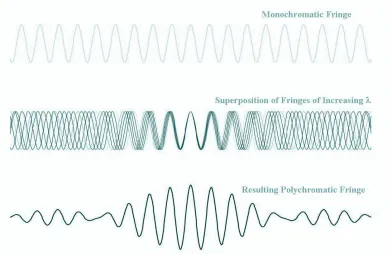
The A given in equation 1.3 is only constant in the case of monochromatic light.
Real interferometric observations are always going to be polychromatic. The intensity
patterns of different wavelengths will have different angular spacings between the
fringes (equation 1.4). When the intensity patterns of interferometric observations
at several different wavelengths are combined, the resulting total intensity pattern is
that of a central “fringe packet” with “side-lobes” extending outward on either side.
This is shown in Figure 1.2. The characterization of this fringe packet can be used
9
Figure. 1.1: Young’s Double-Slit Experiment. Adapted from a figure by H.A. McAl-ister
The observable quantity of an interferometer is the “visibility” of a fringe packet,
defined by Michelson (1920) as:
V = Imax−Imin
Imax+Imin
(1.5)
where Imax and Imin are the maximum and minimum intensity of the interference
pattern, respectively. The visibility derived by an interferometer can be used to
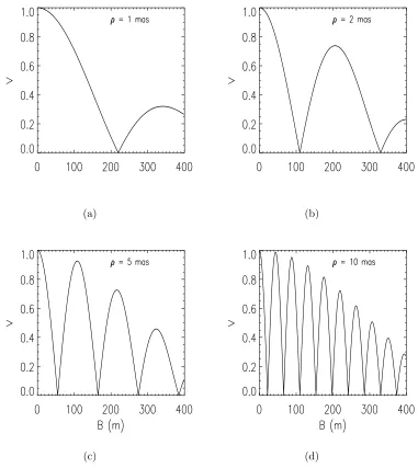
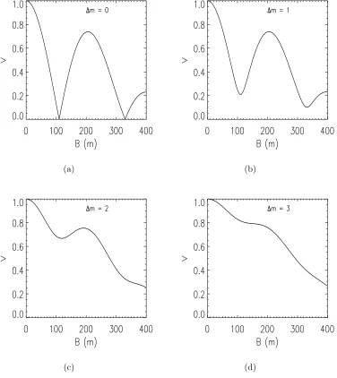
de-termine several parameters of the target system. For single stars, the visibility is
dependent on the star’s angular diameter. For binary systems, the visibility is
de-pend on the angular diameters of the two stars, the separation between them, and
Figure. 1.2: Polychromatic Fringes. These plots show the effects of polychromatic observation. Adapted from a figure by H.A. McAlister
will be discussed later, but depictions of the dependences are shown in Figures 1.3,
1.4, and 1.5. These figures represent the ideal case of monochromatic observation.
Since all observations are polychromatic, the real visibility curves will be affected by
the bandwidth of observation. The resulting curves are the sum of all
monochro-matic curves within the range of the observation bandwidth. This effect, known as
11
(a) (b)
[image:31.612.139.520.181.608.2](c) (d)
13
(a) (b)
[image:32.612.144.520.180.602.2](c) (d)
1.2 The CHARA Array
The sole observation instrument for this project was Georgia State University’s CHARA
Array, located in California on the summit of Mount Wilson. The complete details
of the instrument are given in ten Brummelaar et al. (2005). Six 1-meter telescopes
are spread out on the CHARA grounds in a Y-shaped configuration, producing 15
baselines from 34 to 331 meters. The telescopes are named for their geographic
lo-cation relative to the CHARA’s Beam Combining Laboratory (BCL). The layout of
the telescopes gives six different general baseline orientations (S-E, S-W, E-W, S1-S2,
W1-W2, and E1-E2). The various orientations are of paramount importance to this
project because of their role in SFP observations. The layout of CHARA is presented
[image:33.612.115.536.434.691.2]in Figure 1.6.
15
Light from each telescope is transported as a 12.5-cm diameter collimated beam
through 20-cm diameter evacuated light pipes to the BCL for Optical Path-Length
Equalization (OPLE). The first stage of OPLE involves six parallel tube systems,
referred to as the “Pipes of Pan” (PoPs) that introduce fixed amounts of delay into
the beam (0, 36.6, 73.2, 109.7, and 143.1 meters). Down each PoP line are mirrors
that can be moved into the beam to add or remove fixed amounts of delay. Then,
a variable component of delay must be considered to account for a star’s movement
across the sky during observation. This is achieved by six mobile OPLE carts that
ride on steel rails 46 m in length and provide 92 m of path length compensation.
After the path lengths are equalized, the beams are reduced in size to 1.9 cm in
diameter and split into separate visibile and infrared (IR) wave bands. The visible
part is sent to the tip/tilt system to track the star, while the IR part is sent to the
“Classic” beam combiner for analysis. The layout of CHARA Classic, shown in Figure
1.7, is that of a pupil-plane beam combiner where the two outputs from the beam
splitter are separately imaged onto the Near Infrared Observer (NIRO) camera after
passing through a filter. A filter wheel can be manually rotated through six different
filters, but all observations in this project are taken in K′ (2.1329 µm). Fringes are
detected by dithering a mirror mounted to a piezoelectric translation stage through
a region of delay. The stage is driven with a symmetric sawtooth signal at a data
acquisition rate of 5 samples per fringe for four possible values of the fringe frequency
Figure. 1.7: CHARA Classic. This shows the layout of the CHARA Classic Beam Combiner. Adapted from a figure by H.A. McAlister.
were collected at a rate of 750 Hz for a fringe frequency of 150 Hz.
Almost all observations for this project were conducted using CHARA’s remote
observation facility, the Arrington Remote Operations Center (AROC), located on
the Georgia State University campus in Atlanta. AROC’s computers are connected
to those at CHARA’s Mount Wilson facility through the use of a Virtual Private
Network (VPN), which allows observers to remotely control CHARA’s computers.
From AROC, observers are able to slew telescopes, acquire targets, and initiate the
data collection sequence. With support from the on-site staff at Mount Wilson, AROC
17
– 2 –
Target List
2.1 Observing Criteria
The goal of the observations for this project is the quasi-simultaneous observation
of a target close binary and a calibrator star. The angular separation of the target
and calibrator must fall within a certain range in order to achieve this goal. If the
separation is too large, the two fringe packets will not appear in the same scan over
interferometric delay. If the separation is too small, the two fringe packets could be
overlapping or even unresolved.
The upper limit on the acceptable range of separations is determined by the
specifications of the instrument of observation. Data are recorded with a dither mirror
that oscillates back and forth over a certain range of delay space. The CHARA Array
observation protocol allows the observer to select either a long, medium, or
short-scanning mode. These modes differ in the amount of delay space that is recorded
and the amount of time needed to record each data scan. For the purposes of this
project, the long-scanning mode is the preferred observation mode because it allows
the simultaneous observation of SFPs with larger projected separations. The range
of delay space was 185.62 µm for all data recorded before 2008.
To determine how the separation between two fringe packets in delay space relates
to the angular separation, a scaling equation is used:
ρmas =
206.265 ρµm
Bm
where Bm is the baseline of the observation in meters, ρµm is the separation between
two fringe packets in delay space in µm, and ρmas is the angular separation between
the two packets in mas. The scale depends on which of CHARA’s 15 observation
baselines are being used. For example, using the longest CHARA baseline (S1-E1:
330.67 m), 185.62 µm of delay space equates to 115.79 mas of sky separation. In
2008 January, the range of delay space covered by the dither mirror in long-scan
mode was changed from 185.62 to 142.0µm for operational reasons unrelated to this
project. This new scan range results in an angular distance of 88.6 mas. Conversely,
for the shortest CHARA baseline (S1-S2: 34.08 m) the scan ranges equate to a much
larger portion of the sky: 1123.4 mas pre-2008 and 859.4 mas post-2008. Although
the shorter baseline allows the observer to search a larger portion of the sky, the
resolving ability is much lower, so when creating a target list, the focus is placed on
the scan range available to larger baselines.
When compiling a target list, I looked for targets with a wide orbit semi-major
axis of less than 250 mas. For such targets, an observation baseline can be chosen
such that the projected angular separation is below the upper limit calculated above
on a given night. To accomplish this task, information is needed about both the
target system and the possible baselines of observation. This is explained in detail in
the next section.
There are a few other considerations taken into account when creating the
19
declination limit for objects is -15◦
. Magnitude is a very important factor in a few
different ways. The limiting magnitude of the CHARA Array in K′ band is about
7.5 for the CHARA Classic beam combiner, so only bright targets are available for
observation. Also, two magnitude differences must be taken into account. The
mag-nitude difference between the target close binary and the calibrator wide component
(∆Kwide) affects the amplitude of the fringe packets. If ∆Kwide is too large, the
packet corresponding to the fainter component will not appear at all. Analysis of this
phenomenon will be discussed explicitly in a later section. The other magnitude
dif-ference to consider is between the two stars in the target binary (∆Kclose). If ∆Kclose
is too large, the fringe packet representing the binary will show little to no modulation
in visibility and thus will resemble a single star. The modulation of the visibility is
vital in determining the orbit of the close binary, so a large ∆Kclose disqualifies an
object from being a candidate. A final consideration when choosing a target is the
size of the calibrator. An ideal calibrator is unresolved even on CHARA’s longest
baseline. In general, an angular diameter of 0.5 mas is the cutoff between resolved
and unresolved at CHARA. A collection of the criteria for SCAM targets is given in
Table 2.1.
To find objects suitable for this project, three main sources were consulted: The
Fourth Catalog of Interferometric Measurements of Binary Stars, The 9th Catalog of
Table 2.1. Criteria for Target List
Parameter Limit
Dec. ≥ -15◦
αwide (mas) ≤ 250
K ≤ 7.5
∆Kwide ≤ 3.0
∆Kclose ≤ 2.5
Θcal (mas) ≤ 5.0
2.1.1 The Fourth Catalog of Interferometric Measurements of Binary Stars
The Fourth Catalog of Interferometric Measurements of Binary Stars (Hartkopf et al.
2001) began in 1982 at CHARA by recording all speckle interferometry measurements
taken by the facility’s speckle camera. Later, the catalog expanded to include not
only CHARA’s speckle measurements, but all published speckle, astrometric, and
photometric measurements obtained by high angular resolution techniques. With
this wealth of information, the catalog is a useful resource.
To find possible targets, the entire catalog was searched for any objects with an
angular separation of less than 250 mas at any observation epoch. Unfortunately, this
catalog does not contain explicit multiplicity information (save for a few footnotes),
so the list of possible candidates obtained here was populated by mostly binaries,
21
2.1.2 The 9th Catalogue of Spectroscopic Binary Orbits
One useful source in determining the multiplicity of the targets found in the above
catalog is the 9th Catalogue of Spectroscopic Binary Orbits (Pourbaix et al. 2004).
For the candidate systems, this source was consulted to ensure that there existed
two separate spectroscopic solutions: one corresponding to the wide orbit, the other
corresponding to the close orbit. A certain case could occur in which the close orbit
in the multiple system is the one identified in the above catalog as having an angular
separation less than 250 mas, while the wide orbit’s angular separation is much larger.
These objects are of no interest for the purposes of this project, and this ambiguity can
be resolved by consulting Pourbaix et al. (2004). The spectroscopic orbits contained
within this catalogue are also useful in orbit fitting, which will be discussed in greater
detail later.
2.1.3 The Multiple Star Catalog
The Multiple Star Catalog (MSC) (Tokovinin 1997) is a nearly perfect resource tool
for this project. It is a collection of all known information on hundreds of multiple
systems. All published visual and spectroscopic orbits are presented along with
ref-erences for each. Included with each object is a hierarchical diagram showing the
structure of the multiple system along with the standard naming convention for each
component. Also given are all known magnitudes of the individual components as
value is given for the angular distance between two components in an orbit. This
value is somewhat vague, as the author(s) of the catalog maintain that the exact
meaning of the “separation” depends uniquely on the type of system. Although it is
unclear whether this value refers to either an orbital semi-major axis for the system
or some epoch-specific angular separation, this value does provide a good idea of the
size of the system and whether or not a candidate can be eliminated based on this
criterion. Finally, the spectral types of the individual components are given when
known, as well as the composite spectral types of binary and multiple components.
This catalog contains all of the necessary information to create a target list of
multiple systems. Unfortunately, this catalog was only discovered several months into
this project, otherwise the need for the first two catalogs would have been minimal.
All magnitudes in the MSC are given in V and must be converted to K, which is
close to CHARA’sK′ observing band. Kmagnitudes are estimated using the spectral
types of the individual components andV−K values given in Cox (2000). Conversion
to K gives the overall magnitude as well as ∆Kwide and ∆Kclose, although missing
individual magnitudes and spectral types complicate the process. Although unknown
magnitudes can lead to uncertainty in ∆Kwide and ∆Kclose, these objects are not
rejected as targets. Observation of these objects will reveal whether these objects
should be rejected based on ∆Kwide (absence of secondary fringe packet) or ∆Kclose
(no visibility modulation in the target). The other determination that can be made
23
references listed in the MSC are consulted in order to find radius measurements. If
none are found, the size can be estimated using the spectral type and parallax given
in the MSC and the radii for each spectral type given in Cox (2000). All tertiary
components with an angular diameter greater than 0.5 mas are considered to be too
resolved to serve as good calibrators.
Examination of these catalogs has produced the target list given in Table 2.2.
All of the information given in Table 2.2 has been taken directly from the Multiple
Star Catalog, except for the system K-magnitudes, which were taken from 2MASS
(Skrutskie et al. 2006). Unfortunately, the table has many holes where information
is unavailable. The list is separated into two groups: good targets and marginal
targets, where good targets are loosely defined as those that satisfy most of the
2.2 Observation Planning
When observing SFPs, the separation between the packets is a projected separation
along the particular baseline of observation rather than the intrinsic separation in the
orbit. The projected angular separation ρproj is related to the intrinsic separation ρ
by the following equation:
ρproj=ρ cos(θ−ψ) (2.2)
where θ is the position angle of the wide orbit and ψ is the position angle of the
observation baseline. With knowledge of the wide orbit in the triple system, a suitable
baseline can be selected such that the projected angular separation is below the
threshold determined above for a given epoch.
For the wide orbit, ρ and θ can be calculated for a given epoch using the seven
standard orbital elements for a visual binary. The details of this method are presented
in Appendix A. In addition, the details of the calculation of the baseline lengthB and
baseline position angleψ for a given epoch are found in Appendix A. This information
can be plugged into equation 2.2 to obtainρprojfor the wide orbit in mas for the given
epoch. Thatρprojcan be then plugged into equation 2.1 to determine the separation in
delay space. This information can be used to establish favorable observing epochs and
baselines for any target. As an example, Table 2.3 examines the projected separation
for one target on a single night. The value of ρproj is given in µm for every hour of
the night on every baseline. Because this night is post-2008, any value of ρproj larger
Although in theory, one could observe SFPs at any separation less than or equal
to 142.0µm, in practice, this is not the case. At the limit, the peaks of the two fringe
packets will be separated by 142.0µm, as shown in Figure 2.1. In order to reduce the
data obtained on fringe packets, the entire packets must be visible. To accomplish
this, the coherence length of the fringe packets must be taken into account. The
coherence length is a measure of the length of a fringe packet in the direction of the
motion of the dither mirror, as shown in Figure 2.2. It is determined solely by the
parameters of the instrument and is given by
Λcoh =
λ2
∆λ (2.3)
where λ is the wavelength of observation and ∆λ is the observation bandwidth.
Al-thoughλis a well-known quantity at CHARA (λ= 2.1329µm), ∆λis not. Previously,
a value of ∆λ= 0.250µm had been adopted, but recent estimates by Bowsher (2010)
suggest that the value is closer to 0.350µm. Using these values, the coherent length
is Λcoh = 13.0 µm. Taking into account the size of both fringe packets, the new
maximum tolerable separation to observe SFPs is 142.0 - 26.0 = 116.0 µm. This
separation can be viewed in Figure 2.3.
Drifting of the fringe packets must also be considered. Due to minor
inconsis-tencies in the baseline solution of CHARA, the fringe packets will drift out of the
scanning window over time. Although the cart upon which the dither mirror sits
29
Figure. 2.1: Separated Fringe Packets at Threshold of Simultaneous Observation. These fringe packets are separated by 142.0 microns.
the minor inconsistencies can cause the fringe packets to drift by several hundred
µm per hour. To account for this effect, CHARA’s observation software includes the
“SERVO” tool, which attempts to lock onto a target by finding the highest amplitude
point in a scan, then shifting that position to the center of the scanning window. This
tool is wonderful for observing single fringe packets, but has limited effectiveness for
SFPs. The SERVO will lock onto the higher amplitude packet, moving it to the
cen-ter and pushing the lower amplitude packet outside the window. The observer must
manually move the window to keep the SFPs visible. When issuing the command
to move the window, there is a slight time delay between the computer at AROC
Figure. 2.2: Coherence Length. The distance between the vertical lines represent twice the coherence length of the fringe packet.
continually undershoot or overshoot the proper amount of movement, especially for
fringe packets separated as widely as those in Figure 2.3. This effect can be
com-pounded by poor seeing. Seeing-induced piston variations cause the fringe packets to
oscillate back and forth around their rest position. This oscillation amounts to a few
dozen µm in amplitude, making it nearly impossible to keep both widely separated
fringe packets in the window. Poor seeing is defined as seeing that causes a standard
deviation in the position of a fringe packet larger than 28 µm (20% of the 142 µm
scanning range). Thus, although in theory it is possible to reduce data on fringe
packets of separations near 116 µm, it is impratical to do so. A maximum separation
31
Figure. 2.3: Fully Visible Separated Fringe Packets. These fringe packets are sepa-rated by 116.0 microns.
All of the discussion so far has focused on finding the upper limit of separation. Of
equal importance is the lower limit of separation. At a separation of zero, packets are
blended together, and the individual fringes constructively interfere with each other.
At small non-zero separations, the fringe packets are still blended together. For fringe
packets of equal amplitude, the smallest separation at which the individual packets
can be resolved is roughly 5.1µm. This quantity increases with increasing amplitude
ratio of the fringe packets.
At very small separations, the visibility of each fringe packet is corrupted by the
side lobes of the other packet. The fringes in the side lobes of one packet will either
versa, thus changing the amplitude (visibility) of the packet. The resulting visibility
is not the true visibility of the system. An example of this effect is shown in Figure
2.4. Because the visibility is integral in determining the orbit of the system, observing
SFPs that are close together is unacceptable. Extensive modeling of this “side-lobe
interference” was conducted and is presented in Chapter 4. For now, this effect is
only taken into account in terms of observation planning. The preference here is that
during observations, each packet should lie fully outside of the other packet’s second
side lobe. The second side-lobe is selected as the cutoff point because at this point,
the amplitude of side-lobe interference is roughly at the level of the scatter in the data
in most cases. As with the coherence length, the location of the side lobes of a fringe
packet is determined solely by the parameters of the instrument. The point between
the second and third side-lobes lies at a distance of 32.0 µm from the peak of the
central fringe packet for λ = 2.1329 µm and ∆λ = 0.350 µm. Taking the coherence
length into account, the fringe packets must be separated by 45.0 µm to achieve the
desired separation, as shown in Figure 2.5.
An upper limit (100.0µm) and lower limit (45.0µm) have now been established for
observation purposes. “Separation tables” like Table 2.3 are created for each target
for the 1st and 15th day of each month during the observing season. The separation
values are not substantially different on consecutive nights, so creating separation
tables twice a month is sufficient. Analyzing all the separation tables generated for
33
Figure. 2.4: Side-Lobe Interference. This is an example of side-lobe interference between two fringe packets. The bottom half of the plot shows two model fringe packets as single functions. The top half shows the addition of those two functions and how the visibility amplitudes change from their original value.
targets. In 2009, the decision was made to focus on the targets for which SFPs had
already been observed, which amounted to seven objects (HDs 3196, 35411, 98353,
107259, 129132, 157482, 206901). Parameters of these seven targets, in addition to HD
193322 (an object observed by others and later added to this project), are presented
in Table 2.4. Separation tables for these targets were consulted first when planning
observations. Separations outside of the noted range were considered acceptable for
other targets if the requirements for the main targets had been satisfied.
Most targets can only be observed for a few hours. Examination of Table 2.3
Figure. 2.5: Separated Fringe Packets at Lower Limit of Observation. These fringe packets are separated by 45.0 µm.
to the phenomenon known as baseline rotation, which is similar to aperture synthesis.
As Earth rotates, the baseline’s length and position angle change from the perspective
of the target. Looking at equation 2.2, as ψ changes, ρproj also changes. The other
variables in equation 2.2,ρandθ, change during observation due to orbital movement.
However, the wide orbits for all targets associated with this project are on the order
of years, so the orbital motion during observation is minimal, and changes inρproj are
dominated by baseline rotation.
This observation scheme was first implemented in 2009 with great success. SFPs
were always present when expected and were easily manageable despite the drifting
35
Table 2.4. Targets that produced separated fringe packets
V mag Sp. Type αwide(mas) P (days)
HD No. Name π(mas) wide close wide close wide close wide close
3196 13 Ceti 47.51 6.30 5.60 G0V F8V 241 1.73 2517 2.1
35411 ηOri 3.62 5.65 4.24 B3V B1V 44 0.78 3449 8.0
98353 55 UMa 17.82 5.69 5.39 A1V A1V 91 0.93 1873 2.6
107259 ηVir 6.50 4.20 · · · A2IV 136 7.53 4792 71.8
129132 · · · 6.10 · · · G0III 74 6.69 3385 101.6
157482 V819 Her 14.70 6.11 6.82 G0III F2V 75 0.67 2019 2.2 193322 CHARA 96 · · · 5.97 O9V O8III 67 3.90 11432 312.4
206901 κPeg 4.74 5.04 F5IV F6IV 236 2.81 4240 6.0
difficulty with this scheme is finding a baseline and night on which several targets can
be observed, but for the 2009 and 2010 observing seasons, this was not a problem.
There was concern that the inaccuracy of the published wide orbits might lead to a
ρproj different than what was expected, but, at least for the main targets, this was
not a problem either. Of the seven main targets mentioned earlier, only HD 107259
suffers from a lack of data. This was due to weather conditions and technical issues
with the Array.
Because all pre-2009 data were taken before the observation scheme was put into
effect, many observations during that time featured SFPs outside the necessary range
in separation. These data fall into four categories. First, data in which the separation
is nearly zero show no SFPs, and must be discarded. Second, data in which the
separation is small, but still large enough to show SFPs, may be usable under certain
conditions which will be discussed in Chapter 4. Third, data similar to Figure 2.1,
in which SFPs are visible, but impossible to keep in the scanning window, must be
becomes possible to use the “bracketing” method to collect data. Bracketing involves
37
– 3 –
Data Reduction
The objective in reducing SFP data is to obtain two instrumental visibilities, one for
the target close binary and one for the calibrator wide component. Once these are
obtained, the instrumental visibilities of the wide component can be used to calibrate
the instrumental visilibities of the close binary. The calibrated visibilities of the
close binary can then be used for orbit fitting. Although SFPs have been reduced
extensively for multiplicity studies and determining separations, SFP data have never
been reduced for the purposes of obtaining visibilities from both packets. The data
reduction code used here is a modified form of the MathCAD program “VisUVCalc,”
written by H.A. McAlister and A. Jerkstrand and based on Benson et al. (1995).
The original program directly fits the individual fringes in the packets, determining
V, the visibility of the packet. VisUVCalc also calculates B and ψ for the epoch of
observation.
3.1 Initial data processing
Data sets obtained are standard for observations with the “CHARA Classic” beam
combiner. These files consist of roughly 200 scans of the dither mirror, which oscillates
back and forth through 142.0µm of delay at a frequency of 150 Hz in the region that
the fringe packets are detected. The scan accumulation time is limited to about 5
minutes. In theory, objects could be observed for a longer period of time, but data
CHARA records data using two detector channels, the first of which records the
transmissive component of the beam from one telescope and the reflective
compo-nent of the beam from the other telescope, while the second records the opposite.
CHARA’s detectors record the photon count and the dither mirror position once per
millisecond. The dither mirror positions can be used to break the data into
individ-ual scans by finding every instance in which the mirror changed direction. For the
purposes of data reduction, the x-axis for all scans is left as time in ms, rather than
converting to µm of delay space or mas of angular distance. The recording process
is bookended by shutter sequences (visible in Figure 3.1 as the dips in the flux level)
which help measure the noise levels and the flux ratio between the two telescopes.
The first and third areas of the shutter sequence represent the flux levels of the
in-dividual telescopes. The shutter for one telescope is closed in the first region and
the shutter for the other telescope is closed for the third region. The second region
represents the dark noise scans, where the shutters for both telescopes are closed.
The first step in reducing these data is to account for the dark level, which is
ac-complished by calculating the average flux value from all dark noise scans in both the
“before” and “after” noise scans and subtracting that value from all points in Figure
3.1. Data with the dark noise subtracted is presented in Figure 3.2. After breaking
up the data into individual scans, a low-pass filter can be applied to normalize each
scan, as shown in Figure 3.3. After obtaining the normalized functions of intensity
39
determined. From Benson et al. (1995), the normalized intensities of both detectors
are known:
IA,N(t) = 1 +
2√αβ
α+βV(t) (3.1)
IB,N(t) = 1−
2√αβ
1 +αβV(t) (3.2)
V(t) =V sin(π∆σvgt)
(π∆σvgt)
cos(2πσ0vgt+φ) (3.3)
where α = I2/I1, the intensity ratio between the two telescopes, β = R/T, the
ratio between the reflectance and transmittance of the beam splitter, V(t) is the
visibility as a function of time, V is the visibility amplitude, ∆σ is the inverse of the
coherence length (Λ−1
coh), vg is the group velocity of the dither mirror, t is time, σ0
is the wavenumber, and φ is the phase. By rearranging equations 3.1 and 3.2, the
time-dependent visibility can be written as a function of the intensities of the two
detectors:
V(t) = 0.5(αβ)−0.5( 1
α+β +
1 1 +αβ)
−1(I
A,N(t)−IB,N(t)). (3.4)
The flux reaching the detectors during the shutter sequence allows for the
determina-tion of the quantitiesα and β. When shutter S1 is closed, the flux reaching detector
A, indicated as IAS1, is I2T, while the flux reaching detector B (IBS1) is I2R.
Simi-larly, when shutter S2 is closed, the fluxes reaching detector A and B are, respectively,
41
sequences. For example, to determine the value of IAS1 for a particular data set, the
average of all points in the designated regions in Figure 3.2 is calculated. From the
aforementioned definition of α and β, the following can be derived:
α= IAS1
IBS2
= IBS1
IAS2
(3.5)
and
β = IBS1
IAS1
= IAS2
IBS2
. (3.6)
Once the coefficients αandβ have been determined, a “visibility scan” can finally
be calculated from equation 3.4. Next, the scan is smoothed by isolating the fringe
frequency in the scan’s power spectrum. Taking the Fourier Transform of a scan
gives the characterization of the fringe packets in the frequency domain. The peak
of this power spectrum is ideally located at the frequency set during observation,
which, for this project, is generally 150 Hz, but can occasionally be 100 Hz for fainter
targets. After locating the peak, a bandpass filter of 60 Hz is applied to enhance the
fringe signal relative to the noise present at other frequencies. Bandpass-filtering is
equivalent to multiplying the power spectrum by a box function whose box width is
60 Hz. This enhanced signal is inverse Fourier Transformed to obtain the smoothed
visibility scan. The power spectrum for an example scan has been presented in Figure
3.4 along with the boundaries for the bandpass-filtering. Figure 3.5 shows the results
43
clarity. The bandpass-filtered scan is the final product that is now used to evaluate
the presence of SFPs.
45
Figure. 3.5: Bandpass-filtered scan. The top half of the plot shows the normalized scan in the lower plot of Figure 3.3. After applying the 60-Hz bandpass filter shown in Figure 3.4, the result is the smoothed scan in the lower half of the plot.
3.2 Finding separated fringe packets
The next step is to actually search data for the presence of SFPs. A useful tool in this
undertaking is the fringe envelope. The fringe envelope is obtained by performing a
Hilbert Transform on the visibility scan, in which the negative frequencies are shifted
by -180◦, leaving only the positive frequencies (Farrington et al. 2010). The absolute
value of the resulting inverse transformation is the envelope of the scan. The envelope
of the smoothed scan in Figure 3.5 is shown in Figure 3.6. Shift-and-add co-addition
of many scan envelopes very effectively smooths the atmospheric noise present in the
shift-and-Figure. 3.6: Fringe envelope of a single scan
add procedure involves identifying the maximum of each scan’s envelope, shifting
all of them to the same position on the x-axis, and adding all the scans together.
Instances of poor seeing can cause the secondary packet to move relative to the
position of the primary packet from scan to scan, so that in the shift-and-added
envelope, the secondary packet may be smeared out and not visible. Thus, data must
be meticulously examined in order to confirm or deny the existence of the secondary
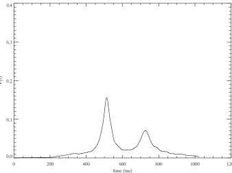
packet. Fig. 3.7 shows a shift-and-added envelope for an entire data set. The primary
packet is prominent, and the secondary packet is clearly visible to the right of the
primary. In cases where the two fringe packets are of similar amplitude, the
[image:65.612.161.504.143.399.2]47
This is due to the possibility of the maximum of the scan switching between the fringe
packets from scan to scan. However, this is not problematic, because the existence of
[image:66.612.162.500.229.481.2]these artifacts still confirms the presence of two fringe packets.
Figure. 3.7: Shift-and-added envelope. The shift-and-added envelope for all non-zero weighted scans in a data set. This envelope represents 86 individual scans.
When the existence of SFPs is confirmed, the next task is pinpointing their exact
locations on the x-axis. The location of a fringe packet is defined as the position
in time of the peak of the packet. Three different methods are used to determine
the positions of the two fringe packets. The method used on a particular data set is
dependent upon the nature of the separation of the fringe packets. The method is
used on each of the scans in the data set. For widely separated packets, like those
performed, one on each side of the marker. The highest amplitude point on each side
is recorded as the fringe packet location.
The second method of finding fringe packet locations is used for SFPs of
interme-diate separation. The higher-amplitude fringe packet (HAFP) is located by searching
the entire scan for the highest point. All scans are then visually inspected to
deter-mine whether this higher amplitude packet is located on the left or right side of the
lower amplitude packet. There is also a special case in which the fringe packets are of
nearly equal amplitude, such that the higher amplitude packet could change between
the left and right packets in successive scans. In any case, the next step is to subtract
the HAFP and search the remaining portion of the scan. The subtraction involves
placing a marker at about 100 ms away from the HAFP’s peak in the direction of the
lower amplitude fringe packet (LAFP). Everything on one side of the marker is set
to zero, leaving only the LAFP. In the special case, markers are placed on each side
of the HAFP at 100 ms, and everything between the markers is set to zero. This is
to ensure that the LAFP is not subtracted out no matter which side it is on. The
highest point remaining is considered to be the location of the LAFP. The location of
the markers, 100 ms, is merely a starting point, and can be changed if the situation
requires it.
The third and final method of finding fringe packet locations is used for very close
and overlapping fringe packets, which will henceforth be known as semi-separated
49
locating the LAFP. In any observation of SFPs, the separation between the two
packets is modified by atmospheric seeing variations such that the fringe packets move
due to differing air path lengths Farrington et al. (2010). A quantitative estimate
this phenomenon, known as piston error, at the CHARA Array is given in Farrington
et al. (2010). The piston error at small separations changes the overall shape of the
fringe packets and virtually ensures that choosing a single value for the location of
the marker relative to the HAFP in every scan is insufficient. Instead of placing a
marker a certain distance away from the HAFP, the location of the marker must be
determined for each individual scan. The trough between the peaks of the two fringe
packets in the scan envelope represents the ideal spot to place the marker. To find
this exact position, the first derivative of the envelope is calculated and the first zero
on the left or right of the peak of the higher amplitude packet is determined. The
location of the first zero corresponds to the trough. The marker is placed here, the
side with the HAFP is subtracted, and the highest point of the remaining portion of
the scan is the location of the LAFP. An example of each type of fringe packet-locating
methods is given in Figure 3.8.
Once the existence of the second packet in a data set has been established and the
locations of each packet determined, each data scan must be examined, and criteria
for the rejection of scans must be established. In order to avoid biasing the results
with low signal-to-noise data, 40% of the scans in each data set are rejected based
Figure. 3.8: Locating fringe packets. The three different methods of locating the second fringe packet in SFP observations. In the upper left plot, a marker (solid line) is placed in the middle of the scan and everything to the left of it is set to zero so that only the smaller packet remains. In the upper right plot, the marker is placed 100 ms to the right of the larger fringe packet, and everything to the left is set to zero. In the bottom plot, the marker is placed at a zero of the first derivative of the envelope of the scan. This is the first zero to the right of the larger fringe packet. Everything to the left of the marker is set to zero.
project by H. A. McAlister. A relative signal-to-noise ratio measurement is calculated
for each scan by dividing the peak of a scan’s power spectrum by the integrated area
under the power spectrum from 300 to 325 Hz (a band outside the position of the
fringe (150 Hz) in the frequency domain). The separation between the two fringe
packets in each scan must also be considered. If the separation measurement for a
51
of the fringe packets has been misidentified, most likely due to noise peaks. These
scans are rejected. A related consideration is the position of the fringe packets. The
positions of the packets should be relatively consistent between successive scans in a
data set. To measure the level of consistency, the position of one fringe packet in a
scan is compared to the mean of that packet’s position in the two previous and the
two successive scans. If the position differs from that mean by more than 100 ms, this
fringe packet is considered to be misidentified, and the scan is rejected. This process
is repeated for the other fringe packet. Finally, all scans are visually inspected to
make sure that both fringe packets are still within the scan range. Due to either poor
seeing or the general inconsistency in the optical path-length equalization, the fringe
packets may drift out of the scan range during observation. Scans such as these must
be rejected as well. Typically, after all rejection criteria have been satisfied, roughly
50% of the data scans remain.
3.3 Fringe fitting
Instrumental visibilities are obtained for a data set by determining the instrumental
visibility of a packet in each individual scan, then averaging all of those values. It
should be noted that because of the changing baseline and atmospheric effects,
vis-ibilities cannot be determined by coadding the individual fringe packets from each
scan and deriving a visibility value from the coadded data (Benson et al. 1995). In