PERFORMANCE ANALYSIS OF SMART ANTENNA BASED ON MVDR
BEAMFORMER USING RECTANGULAR ANTENNA ARRAY
Suhail Najm Shahab
1, Ayib Rosdi Zainun
1, Nurul Hazlina Noordin
1, Ahmad Johari Mohamad
1and
Omar Khaldoon A.
21Faculty of Electrical and Electronics Engineering, Universiti Malaysia Pahang, Pahang, Malaysia 2School of Computer and Communication Engineering, University Malaysia Perlis, Malaysia
E-Mail: [email protected]
ABSTRACT
The performance of smart antenna system greatly relies on the beam forming technique that forming the main lobe beam pattern to the desired user direction and place null in the direction of undesired interference source. This paper investigates the implementation of Minimum Variance Distortionless Response (MVDR) Adaptive Beam-Forming (ABF) algorithm on Rectangular Antenna Array (RAA) is discussed and analyzed. The MVDR ABF technique performance is studied in accordance with varying the number of array elements, spacing between the array elements, the number of interference sources, noise power label, and the number of snapshots. The MVDR performance is compared on the basis of output radiation pattern and SINR. Computer simulation results show that the performance of the MVDR improved as the number of elements get more. This mean MVDR strongly depends on the number of the element. 0.5λ is considered the best spacing between adjacent antenna elements, the performance degraded as the noise power label increased, and more accurately resolution occurred when the number of snapshots increased.
Keywords: beamforming, minimum variance distortionless response, rectangular antenna array, smart antenna.
INTRODUCTION
Most beam forming techniques have been considered for using at the base station (BS) since antenna arrays are not feasible at mobile terminals due to space limitations [1].
The Long Term Evolution (LTE) as defined by the 3rd Generation Partnership Project (3GPP) is a highly flexible radio interface, its initial deployment of LTE is in 2011. LTE is the evolution of 3GPP Universal Mobile Telecommunication System (UMTS) towards an all-IP network to ensure the competitiveness of UMTS for all next ten years and beyond. LTE was being developed in Release 8 and 9 of the 3GPP specification. According to Maravedis anticipates that 3 LTE-TDD and 59 LTE- FDD networks will be operational worldwide by the end of 2011. There will be 305 million LTE subscribers by 2016, which is about 44 million (14%) will be TDD-LTE users, and the rest 261 million (86%) will be FDD-LTE. [2]. With increasing trend of the number of subscribers and demand for different services in wireless systems, there are always requirements for better coverage, higher data rate, improved spectrum efficiency and reduced operating cost. To fulfill these requirements, beamforming technique able to focus the array antenna pattern into a particular direction and thereby enhances the signal strength.
Interference is one of the significant obstacles in wireless communications. The interference can be caused by the signal itself or by other users [3]. The signal can interfere with itself due to multipath components, where the signal is gathered with another version of the signal that is delayed because of another propagation path. The fundamental principle of ABF is to track the statistics of the surrounding interference and noise field and adaptive-ly search for the optimum location of the nulls that can most significantly reduce the interference and noise under
the constraint that the desired signal is not distorted at the beamformer’s output [4].
The basic idea of the MVDR algorithm is to esti-mates the beamforming coefficients in an adaptive way by minimizing the variance of the residual noise and interference while enforcing a set of linear constraints to ensure that the desired signals are not distorted [4]. The authors in [5] proposed an enhanced model of MVDR al-gorithm by changing the position of the reference element in steering vector to be in the middle of the array with an odd number of elements. Simulation results showed that modified MVDR has a realistic behavior, especially for detecting the incoming signal’s direction and outperforms the conventional MVDR. The signal to interference plus noise ratio (SINR) maximization is one of the criterion employed in joint transmitter and receiver BF algorithms [6, 7]. In [8] mentioned that the element spacing must be d ≤ λ/2 to prevent spatial aliasing. In [9] the author presents a comparative study of minimum variation distortionless algorithm and Least Mean Square (LMS) algorithm. Results indicated that LMS is a better performer.
www.arpnjournals.com
produced in the directions of unwanted signals that symb-olize co-channel interference from mobile users in the adjacent cells. Before adaptive beamforming, the directi-on of arrival estimatidirecti-on is used to specify the main direct-ions of users and interferers. The function of ABF algorithm is used to direct the main beam towards look direction and nulls towards jammer directions.
So far, ABF is a function of the number of elem-ent, spacing between adjacent elements, the angular sepa-ration between Signal-of-Interest (SOI) and Signal-Not-of-Interest (SNOI), noise power level and number of sna-pshots. Therefore, it is important to investigate the impact of these parameters on the radiation pattern of an antenna array that able to offer the best BF capabilities in term of directing the main beam toward the direction of the SOI while placing nulls towards the direction of SNOI. This work includes simulation results and performance anal-ysis of MVDR algorithm with rectangular antenna array. The analysis of the MVDR in this work is in four scenarios where the MVDR performance is evaluated with two important metrics; beampattren and SINR. This analysis does not only help us better understand the MVDR beamformer but also help us design better array systems in practical application. The remainder of this pa-per is organized as follows. In section III, beamformer design method is described. The simulation setup and the numerical outcomes obtained, and discussion are provi-ded in Section IV. At last, Section V concludes the paper.
METHODOLOGY
The mathematical formulation of the design model for adaptive beamforming will be presented in det-ail in this section. Let there is S desired signal and I interference sources transmitting on same frequency cha-nnel simultaneously. The algorithm starts by constructing a real-life signal model. Consider a number of plane wav-es from K narrowband sourcwav-es impinging from azimuth and elevation angles (θ,ϕ), the impinging radio frequency signal reaches into the antenna array from a far field to the RAA geometry. If the interelement distance is constant, it is called Uniform Rectangular Array (URA).
Figure-1 show a rectangular antenna array placed on the x-y plane. There are N elements in the x-direction and M elements in the y-direction creating an N×M array of identical elements. The n-mth element has weight wnm. The x-directed elements are spaced dx apart, and the y-directed elements are spaced dy apart. The rectangular array can be viewed as N linear arrays of M elements or as M linear arrays of N elements.
Figure-1. Rectangular antenna array geometry [10].
The total signals received by an adaptive antenna array at time index, t, become:
Ii
n i
S
s s
T
t
x
t
x
t
x
x
1 1
)
(
)
(
)
(
(1)
I
i
n i i i s
s S
s
s t a x t a x
x
1 1
) , ( ) ( )
, ( )
(
(2)Where xs(t), xi(t),xn(t), denote the desired signal, interference signal and noise signal added from White Gaussian noise, respectively. The unwanted signal consis-ts of xi(t)+xn(t,), the desired angle and interference direct-ion of arrival angles are (θs,ϕs) and (θi,ϕi), respectively. a(θs,ϕs) denote the steering vector for wanted signal while a(θi,ϕi) refer to the interference signal steering vector.
Steering vector is a complex vector containing responses of all elements from the array to a narrowband source of unit power depending on the incident angle, it is given as [11]:
N
n M
m
md nd
jq M
N
y x
e
a
1 1
)) sin( ) sin( ) cos( (
)]
,
(
[
(3)T L a a a a
A[ 0, 1, 2,... 1]
Where j is the imaginary unit of a complex number, (i.e. j2 = -1), q=2π/λ is the wave number, λ is the wavelength of the received signal, (θ,ϕ) composed of azimuth angle
[0, 2π] and elevation angle
[0, π/2] while A denotes the matrix form of the steering vector and (.)T denote the transposes operators.The signal xT(t) received by multiple antenna elements is multiplied by a series of amplitude and phase (weight vector coefficients) which accordingly adjust the amplitude and phase of the incoming signal. This weight-ed signal is a linear combination of the data at N×M ele-ments, resulting in the array output, y(t) at any time t, of a narrowband beamformer is given as:
)
(
)
(
t
w
x
t
y
TH nm
(4)
CN×M beamforming complex vector. (.)H denotes the conjugate transpose (Hermitian transpose) for a matrix.The weight vector at time t + 1 for any system that uses the immediate gradient vector ∇𝐽(t)for weight vector upgrading and evades the matrix inverse operation can be written as follows:
)] ( [ 2 / 1 ) ( ) 1
(t W t J t
W
(5)where 𝜇 is the step size parameter, which controls the speed of convergence and lies between 0 and 1. While the smallest values of 𝜇 facilitate the high-quality estimation and sluggish concurrence, the huge values of it may result in a rapid union. However, the constancy over the minimum value may disappear. Consider
1/0 (6)
An instantaneous estimation of gradient vector is written as: ) ( ) ( 2 ) ( 2 )
(t p t Rt W t
J
(7)
)
(
)
(
)
(
t
d
*t
x
t
p
T (8))
(
)
(
t
x
t
x
R
y
T TH (9)An precise calculation of ∇𝐽(t) is not possible because prior information on cross-correlation vector, 𝑝
and covariance matrix, 𝑅y of the measurement vector are
required. By substituting (7) into (5), the weight vector is derived as follows:
) ( ) ( )] ( ) ( ) ( )[ ( ) ( )] ( ) ( ) ( [ ) ( ) 1 ( * * t e x t W t W t x t d t x t W t W t R t p t W t W T T T
(10)The desired signal can be further defined by the following three formulas:
)
(
)
(
)
(
t
w
t
x
t
y
TH
(11)) ( ) ( ) ( ) 1 ( ) ( ). ( ) ( * t e t x t W t W t y t d t e T
(12)The covariance matrix, Ry is constructed conventionally with unlimited snapshots. However, it is estimated by using limited snapshots signal in actual application. It can be expressed as:
) , ( ) , ( 2 s s H s s s
s a a
R
(13)M N n i i H I i i i i n
i
a
a
Id
R
21 2
)
,
(
)
,
(
(14))] ( ) ( [x t x t R
R
Ry s in T TH (15)
where Ry,
2
s
,
i2,
n2, IdL, Rs, Ri+n and E[.] denotes, res-pectively, the theoretical covariance matrix, power of the desired signal, interference power, noise power, identity matrix, SOI covariance matrix,interference plus noise covariance matrix and expectation operator.
The common formulation of the MVDR beamfo-rmer that determine the N×M optimum weight vector is the solution to the following constrained problem [12]:
] ) ( [ min y t 2
1 ) , ( . . } { ) , ( min s s H y H w a w t s w R w P
(16)where P(θ, ϕ)denote the mean output power, a beam pattern can be given in dB as [13]:
) , ( max ) , ( log
20 10 P P pattern
beam (17)
This technique minimizes the contribution of the undesir-ed signal by minimizing the power of output noise and interference and ensuring the power of useful signal equal to 1 in the real user direction wHa(θ
s,ϕs)=1. By using Lagrange multiplier, the MVDR weight vector that give the solution for above equation as following formula [14]:
) , ( ) , ( ) , ( 1 1 MVDR s s y s s H s s y a R a a R w
(18)
Inserting (19) into (11), the output of MVDR beamformer is given by
n H i i i H s n H i i i H s s s H T H
x
w
a
t
x
w
t
x
x
w
a
t
x
w
t
x
a
w
t
x
t
w
t
y
)
,
(
)
(
)
(
)
,
(
)
(
)
(
)
,
(
)
(
)
(
)
(
(19)The output signal power from the array as a function of the DOA estimation, using optimum weight vector from MVDR beamforming method [15], it gives by MVDR sp-atial spectrum for angle of arrival estimated by detecting the peaks in this angular spectrum as [16]:
) , ( ) , ( 1 ) ( 1 s s y s s H MVDR a R a P
(20)Finally, the SINR defined as;
I i n i s SINR 1 10 log 10
(21)SIMULATION RESULTS AND DISCUSSION
www.arpnjournals.com
[image:4.595.311.543.260.391.2]number of elements separated by inter-element spacing, d, at carrier frequency (Fc) of 2.6 GHz, which is the spec-trum band is allocated for LTE operators in Malaysia [17]. To measure the performance of the MVDR algorith-m for ABF applications with varying parameters such as the number of elements in the array, distance between the adjacent elements, number of SNOIs, accuracy to disting-uish interference in the location very close to the SOI, the number of snapshots (ns), and noise power, σn. The goal is to analysis the effect of parameters mentioned above that achieved the best beamforming capabilities to form the main beam in wanted direction and place null in the directions of interference with highest SINR output. Four different scenarios are considered, and the simulation parameters setting in this paper are shown in Table-1.
Table-1. Simulation parameters.
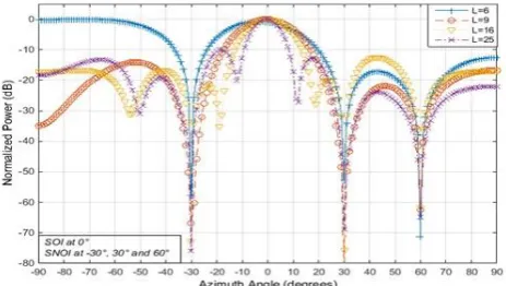
a) The first scenario
First simulation scenario depicted the results calculated by considered the distance between array elem-ents set to be dx=dy=d=0.5λ as usually used in the most MVDR algorithm. Uniform RAA with N×M = 6 isotropic elements of [N=3, M=2], 9 isotropic elements of [N=3, M=3], 16 isotropic elements of [N=4, M=4], and 25 isotr-opic elements of [N=5, M=5] elements, the additive noise is modeled as a complex zero-mean white Gaussian noise. Three interfering sources are assumed to have Direction of Arrivals (DOAs), θi ±30º and 60º with ϕi = 0º respectively. The desired signal arrival is considered to be a plane wave from the presumed direction (0º, 0º). To im-prove the signal performance of the desired target and nullifying interference directions by using the MVDR BF technique. Figure 2 shows a typical 2D beam pattern plot displayed in the rectangular coordinate, it demonstration the effects if the number of elements is increased for SOI at (0°, 0°) and
SNOIs at (±30°,0°) and (60°, 0°) respectiv-ely. This simulation was repeated for 6, 9, 16, and 25 elements with an input SNR of 10dB and 300ns. The plots observe that the MVDR successfully form nulls at each of the income interference sources, and it provide maximum gain to the look direction of the desired user direction. Moreover, increasing the number of elements resulting in the width of the main lobe decreases and the number of nulls in the pattern increases. The number of side lobes (SLs) increases as well the level of the first and subsequent SLs decreases compared to the main lobe. SLs represent power radiated in potentially unwanted directio-ns so in a wireless communications system, SLs will con-tribute to
the level of interference spread in the cell by a transmitter as well as the level of interference seen by a receiver when antenna arrays are used. The main lobe be-amwidth (MLBw), maximum side lobe level (MSLL) that is closest to the main beam, maximum depth null (MDN) at interference direction and output SINR are shown in Table 2. On the other hand, the computing operations be-come more complex. Besides, as the number of elements increases, the mean cost of design increases due to the increasing number of RF modules, A/D converters, and other components. This causes the operational power con-sumption to increase too.
[image:4.595.52.287.307.422.2]Figure-2. Beam pattern analysis of MVDR varying N×M = 6, 9, 16, and 25 with d=λ/2.
Table-2. MVDR performance analysis for SOI at 0° and
SNOIs at ± 30º and 60º with varying N×M at d=λ/2.
b) The second scenario
The distance between the antenna sensors is an important factor in the design of an antenna array. Second simulati-on scenario illustrates the results that calculated by consi-dering N=4, M=4, with interelements spacing of
dx=dy=d = λ/8, λ/4, λ/2, and λ for SOI at (0°, 0°) and SNOIs at (±30°, 0°) and (60°, 0°).
[image:4.595.309.545.463.561.2]bigger than λ/2, causes grating lobes that degrade the MVDR performance also. Therefore, the elements have to be far enough to avoid mutual coupling, and the spacing has to be ≤ λ/2 to avoid grating lobes. As the spacing bet-ween elements increases the main beam width decreases resulting in higher directivity, the number of SLs also increases and highest output SINR obtained by λ/2 due to greatest interference suppression as depicts in Table-3.
Figure-3. Beam pattern analysis of MVDR varying d = λ/8, λ/4, λ/2, and λ with N×M =16.
Table-3. MVDR performance analysis for SOI at 0° and
SNOIs at ± 30º and 60º with different d and N×M =16.
c) The third scenario
Using multiple antennas at the BS can reduce the effects of co-channel interference, multipath fading, and backgr-ound noise. Many BF algorithms have been devised to cancel interference sources that appear in the cellular sys-tem. MVDR algorithm can null the interferences without any distorted to the desired path.
The third simulation scenario demonstrates the MVDR behavior when the number of SNOIs increased. The subsequent MVDR pattern plotted with cancelation for all interferences is shown in Figure-4. It shows a beam pattern for a 16 element rectangular array in the presence of different angle of arrival (AoA) for SOI and SNOIs. In figure-4, the output of MVDR BF algorithm is illustrated against a different number of interference sources as tabl-eted in Table-4. It can be seen that the performance of the MVDR is affected by the number of SNOIs as the numb-er of intnumb-erfnumb-erence increases, the SINR decrease. In case of two interference sources, it is found that the deep null of -66.6dB comparing to -48.5dB for 16 elements for a study conduct by [18] based on conjugate gradient metho-d ABF algorithm. For 4 interference sources, the MVDR was able to form the main beam to reach a desired directi-on even for closest interference to the user which means better
result is obtained when the angular separation between the SOI and SNOI increases.
Figure-4. Beam pattern analysis of MVDR, N×M = 16 and d=λ/2 with different SOI and SNOIs AoAs.
Table-4. Comparison of SINR values for N×M =16 and d=λ/2 with different SOI and SNOIs AoAs.
d) The fourth scenario
In this scenario, compares the effect of various noise po-wer levels, σn, and different number of snapshots, ns, on the performance of MVDR for a desired user at 0° and three interference signal at ± 30º and 60º with N=4, M=4, d=λ/2. Figure-5 give the output beam pattern with four different noise power ranging from -40dB to 40dB. It can be seen that the four curves are noticeably very similar, the MVDR shows better SINR of 92.4dB at a noise power level of -40dB with null all interference sources as demo-nstrated in Table-5. The output SINR decreases as the noise power increases. However, the reduction (null power) at higher values of σn is much less than at lower values of σn and the performance of the MVDR algorithm deteriorates as the noise power increases.
www.arpnjournals.com
Figure-5. Beam pattern analysis of MVDR varying σn = ±10, and ±40dB with N×M =16, d=λ/2.
Figure-6. Beam pattern analysis of MVDR varying ns = 10,50,250, and 500 with N×M =16, d=λ/2.
Table-5. MVDR performance analysis for SOI at 0° and
SNOIs at ± 30º and 60º with different
n at N×M =16 and d=λ/2.Table-6. MVDR performance analysis for SOI at 0° and
SNOIs at ± 30º and 60º with different ns at N×M =16 and d=λ/2.
As seen from Table-5, the main lobe beamwidth (MLBw) remain almost the same and maximum side lobe level (MSLL) slightly change as σn increases, while the nulling level and SINR strongly affected with σn
increases. In addition, Table-6 shows the SINR increases as ns increases owing to the increasing probability of finding a better solution. In other words, sharper and deeper nulls would be produced and hence improve the SINR through increasing number of snapshots.
CONCLUSIONS
MVDR adaptive beamforming algorithm with rectangular antenna array geometry has been evaluated in this paper. Different scenario’s cases are considered to pr-ovide a maximum signal to interference plus noise ratio (SINR) for the desired user direction by placing deepen nulls at directions of the interfere source in the radiation pattern. This paper shows the influence of a different nu-mber of antenna elements, different inter element spacing, different number of interference sources with varying an-gular separations between SOI and interferences, different label of noise power, and different number of snapshots on MVDR beam pattern and SINR. The MVDR beamformer demonstrated its ability to direct the antenna main beam in the direction of the desired user as well as its ability to place null the interference source. The presented results show that when antenna elements are more, the main lobe beamwidth become smaller resulting in higher system capacity. Meanwhile, the drawback is increasing cost, size and complexity. It is found that λ/2 is the best element spacing [18] for avoiding grating lobes, mutual coupling effects, and better depth null performance. MV-DR rejects with very low power level, and good accuracy can be obtained even in the case of multiple interferences. The noise level is an important factor that affects the MV-DR performance. Increases number of snapshots resulting higher SINR and more accurate main beam pattern. The computation time can be further decreased, if higher signal processor is used. An ongoing research extends the results of this paper to enhanced MVDR.
REFERENCES
[1] Liberti J. C. and Rappaport T. S. 1999. Smart antennas for wireless communications: IS-95 and third generation CDMA applications. Prentice Hall.
[2] Garza C. 2011. 4G Digest - 17.25 million BWA/WiMAX and 320 thousand LTE subscribers reached in Q1 2011 in 4G Digest.
[3] Halim M. A. 2001. Adaptive array measurements in communications. 1st ed. Artech House Publichers. Norwood, MA, USA.
[4] Pan C., Chen J. and Benesty J. 2014. Performance study of the MVDR beamformer as a function of the source incidence angle. IEEE/ACM Transactions on Audio, Speech, and Language Processing. Vol. 22, No. 1, pp. 67–79.
performance using modified minimum variance distortionless response beamformer algorithm, The Second International Conference on Electronic Design (ICED). pp. 198–203.
[6] Choi R. L.-U., Murch R. D. and Letaief K. 2003. MIMO CDMA antenna system for SINR enhancement. IEEE Transactions on Wireless Communications. Vol. 2, No. 2, pp. 240¬¬¬¬¬¬–249.
[7] Serbetli S. and Yener A. 2004. Transceiver optimization for multiuser MIMO systems. IEEE Transactions on Signal Processing. Vol. 52, No. 1, pp. 214–226.
[8] Manolakis D. G., Ingle V. K. and Kogon S. M. 2005. Statistical and adaptive signal processing: spectral estimation, signal modeling, adaptive filtering, and array processing. Artech House, Inc. Norwood, MA, USA.
[9] Das K. J. and Sarma K. K. 2012. Adaptive Beamforming for Efficient Interference Suppression Using Minimum Variance Distortionless Response. International Conference on Advancement in Engineering Studies & Technology. pp. 82–86.
[10] Gross F. 2015. Smart antennas with MATLAB: principles and applications in wireless communication. 2nd ed. McGraw-Hill Professional.
[11] Allen B. and Ghavami M. 2005. Adaptive array systems: fundamentals and applications. John Wiley & Sons.
[12] Souden M., Benesty J. and Affes S. 2010. A study of the LCMV and MVDR noise reduction filters. IEEE Transactions on Signal Processing. Vol. 58, No. 9, pp. 4925–4935.
[13] Godara L. C. 1997. Application of antenna arrays to mobile communications. II. Beam-forming and direction-of-arrival considerations. Proceedings of the IEEE. Vol. 85, No. 8, pp. 1195–1245.
[14] Renzhou G. 2007. Suppressing radio frequency interferences with adaptive beamformer based on weight iterative algorithm. In Conference on Wireless, Mobile and Sensor Networks, (CCWMSN07), IET.
[15] Haykin, S. 2013. Adaptive Filter Theory. 4th ed. Prentice Hall.
[16] Capon J. 1969. High-resolution frequency-wavenumber spectrum analysis. Proceedings of the IEEE. Vol. 57, No. 8, pp. 1408–1418.
[17] Malaysian Communications and Multimedia Commission. 2011. SKMM-MCMC Annual Report. ;
Available from:
http://www.skmm.gov.my/skmmgovmy/media/Gener al/pdf/.