A Predator prey Model with Predator Population Saturation

A Predator-prey Model with Predator

Population Saturation

Quay van der Hoff

1,*

_{, Temple H. Fay}

2

1_{Department of Mathematics and Applied Mathematics, University of Pretoria, South Africa} 2_{Department of Mathematics and Statistics, Tshwane University of Technology, South Africa}

Copyright©2016 by authors, all rights reserved. Authors agree that this article remains permanently open access under the terms of the Creative Commons Attribution License 4.0 International License

Abstract

In this article, a new predator-prey model having predator saturation is proposed. The model resembles a classical Rosenzweig-MacArthur type model, but comes with an added function, the population saturation function of the predator. This function of the predator population is a factor in the predator fertility term in the model. Consequently the model behaves better than the Rosenzweig-MacArthur model since all solutions are bounded within the population quadrant. An invariant region arises where the Poincaré-Bendixon theorem can be applied. In most cases there is but a single critical value, either an attracting spiral point suggesting a stable population pair or an unstable node, resulting in a unique limit cycle. This model is fully described and an analysis of the stability of critical values is provided. The robustness of the model is demonstrated based on the classification of Gunawardena [8].

Keywords

Predator-prey Model, Predator Saturation, Poincaré-Bendixon Theory, Limit Cycles

1. Introduction

There is a multitude of predator-prey models in the literature. These models originated with those of Lotka [12] (1925) and Volterra [15] (1931) and have been much refined, since then. In this paper an original predator-prey model, referred to as the FGH model, is proposed and each term has a firm ecological basis for its inclusion and form.

The model is, in essence, a classical Rosenzweig-MacArthur [14] type model with an added function which is called the population saturation of the predator. As this model has bounded solutions in the population quadrant, Poincaré-Bendixon theory [16] applies. That is, bounded solutions in conjunction with a unique unstable equilibrium in the population quadrant, ensures the existence of at least one periodic solution. The long-term

steady states are determined, as well as the long-term behaviour's dependence on initial conditions. In particular, it is shown that the FGH model, with specific parameter values, has equilibrium values which lead to either limit cycles or attracting spiral points.

2. The FGH Model

In this section, the component functions in the FGH model are described in modeling perspective. It is shown that all solutions originating in the population quadrant (

x

>

0

,

y

>

0

) remain bounded. Formulas for the determination of equilibrium points are derived.

2.1. Functions Comprising the FGH Model Consider a predator-prey model of the form:

)

(

)

(

)

(

)

(

)

(

)

(

)

(

)

(

y

h

y

x

p

y

y

x

p

y

x

g

x

x

x

ε

h

x

φ

+

=

−

=





(1)

where

x

(

t

)

denotes the number of prey and

y

(

t

)

denotes the number of predators at given time t. The functions

h

x

φ

,

g

,

p

,

,

and h are continuously differentiable and defined for all

t

≥

0

such that existence and uniqueness conditions are satisfied for initial value problems.

in form to

(

1

−

x

/

K

)

so that

φ

(

x

)

g

(

x

)

is similar to the logistic growth introduced by Verhulst [19]. To generalize the classical logistic growth it is assumed that

g

(

x

)

is positive over an interval

[

0

,

K

)

with

g

(

K

)

=

0

and

0

)

(

x

<

g

for

x

>

K

. The positive constant

K

is the carrying capacity for the prey. A variety of forms for

g

(

x

)

have all been proposed, for example see Chen and Xie [10], and Huang, Wang and Zhu [9].

The function

p

(

x

)

x

(

y

)

represents the predation rate of the predator population y on the prey population x. Generally, the function

p

(

x

)

is a Holling type I, II or III functional response. This functional response is bounded above by some constant a and below by the linear function

K

x

K

p

(

)

/

. It is argued below that there is no loss of generality to assume that

x

is always less than

K

, thus

a

x

p

K

x

K

p

(

)

/

≤

(

)

≤

for all

x

in the interval

[ ]

0,K . The function

p

(

x

)

may take on many forms, such as the

)

arctan(

ax

, as proposed by Attili and Mallak [1] or )

1

( _−e−ax _{, which is known as Ivlev's functional response [11].}

The increasing function

x

(

y

)

is the predation rate of the predator and is bounded by two linear functions,

Sy

sy

and

, where s is the minimal predator efficiency and S the maximal predator efficiency, so that

.

)

(

y

Sy

sy

≤

x

≤

This function, therefore behaves much the same as

φ

(

x

)

.

On the other hand,

h

(

y

)

is a decreasing function representing the mortality rate of the predator in the absence of prey. Let

γ

denote the minimal mortality rate and

Γ

the maximal mortality rate. Therefore, −Γy≤

h

y≤−

γ

y. The function

p

(

x

)

x

(

y

)

h

(

y

)

represents the conversion of prey to fertility for the predator. The term

h

(

y

)

behaves similarly to

g

(

x

)

; it is assumed that

h

(

y

)

is positive over an interval

[

0

,

L

)

, where

h

(

L

)

=

0

and

h

(

y

)

negative for

y

>

L

. This means that

x

(

y

)

h

(

y

)

closely resembles a logistic growth function, which is zero at

L

y

y

=

0

and

=

, positive over the interval

(

0

,

L

)

and negative if

y

>

L

. The constant

L

is called the population saturation of the predator. For small populations of the predator there is positive growth (due to the predation), but if the population of the predators becomes too large, the predator population begins to decline and will decrease until it becomes less than

L

. The maximum value of

)

(

)

(

y

h

y

x

over

[

0

,

L

]

will be denoted by H.

That predators can become less efficient at converting prey biomass to predator biomass as their population increases, is validated by a study conducted by Schmidt and Mech [13] on the optimal wolf pack size. All the data they collected suggested that there was less food per wolf as pack size increased and accordingly the pack size decreased. They use the term "optimal pack size” which is equivalent to

population saturation L in the FGH model.

From the discussion above, assume with regards to System (1) that:

(H1) g(0)>0 and there exists a K >0 so that

0 ) (x >

g over the interval [0,K .)

Furthermore, g(K)=0, and g(x)<0 for x>K. (H2)

φ

(

0

)

=

0

,

φ

('

x

)

≥

0

and there exist positive constants r and R so that

rx

≤

φ

(

x

)

≤

Rx

for all x in the interval

[

0

,

K

]

. Similarly,

0

)

0

(

=

p

and

p

('

x

)

≥

0

and there exists a positive constant

a

so that

p

(

K

)

x

/

K

≤

p

(

x

)

≤

a

for all x in the interval

[

0

,

K

]

.

(H3)

x

(0)=0 and x('y)≥0 and there exist positive constants s and S so that

sy

≤

x

(

y

)

≤

Sy

for all

y

>

0

. Similarly,

0 ) 0 ( =

h

and

h

('y)<0 and there exist positive constants

γ

and Γ so that

−

Γ

y

≤

h

y

≤

−

γ

y

for all

0

>

y

and finally, 0

) 0 ( >

h and there exists an

L

>

0

so that h(y)>0 over the interval [0,L),

h

(

L

)

=

0

, and h(y)<0for y>L.

2.2. The Invariant Region of the FGH Model

Let

x

(

t

)

and

y

(

t

)

be solutions of System (1). It is argued that under the assumption (H1), that is

g

(

x

)

similar in form to (1−x/K) , then the solution

x

(

t

)

remains less than

K

as

t

→

∞

.

First note that if x(0)≥K, then

g

(

x

)

<

0

, resulting in

0

<

x



. Therefore

x

(

t

)

is decreasing and will continue to decrease until

x

(

t

)

is less than

K

. The interaction between

φ

(

x

)

g

(

x

)

and

p

(

x

)

x

(

y

)

may permit

x



to change sign so that

x

(

t

)

may start increasing. However,

)

(

t

x

can now never become as large as

K

again, since

x



is negative at

K

requiring x to go through another sign change before

x

(

t

)

reaches

K

. Therefore each time

)

(

t

x

approaches

K

, it starts decreasing again resulting in oscillating behaviour. Similarly, if x(0)<K,x(t) can never reach

K

, so that

x

(

t

)

is bounded by

K

as

∞

→

t

. Consequently it can be assumed that

∞

→

<

<

x

(

t

)

K

as

t

0

. A similar argument applies to

starting in the rectangle

[ ] [ ]

0,K × 0,L will remain within the rectangle, an invariant region for System (1).

2.3. Equilibrium Points

The equilibrium points of System (1) are values of

y

x

and

for which

x



=

0

and

y



=

0

. To exclude the possibility of extinction of both species, assume

0

)

(

and

0

)

(

x

≠

h

x

≠

φ

. To find the equilibrium points

we observe:

If

x



=

φ

(

x

)(

g

(

x

)

−

p

(

x

)

x

(

y

)

/

φ

(

x

))

=

0

,

then

. 0 ) ( ) ( ) ( )

( − y =

x x p x

g

x

φ

(2)

If

y



=

h

(

y

)(

1

+

ε

p

(

x

)

x

(

y

)

h

(

y

)

/

h

(

y

))

=

0

,

then

. 0 ) ( ) ( ) ( ) (

1+ =

y y h y x p

x

_h

ε

(3)

It will be assumed that equations (2) and (3) each have at least one positive solution, and there exists at least one

(

K

)

x

*

_∈

0

,

_and

_y

*

_∈

( )

₀

_,

_L

_{satisfying both equations} simultaneously.

3. Special Case of the FGH model

Consider, as a special case of the FGH model, the system

      −       + + − =       + −       − = L y H x xy y y H x xy K x rx x 1 1 ε γ α   (4)

which contains the conventional logistic term

)

/

1

(

x

K

rx

−

and a Holling type II functional response

)

/(

x

H

x

+

α

. The constant

L

is introduced as the saturation population of the predator in the same way as the

K

represents the carrying capacity of the prey. The intrinsic growth rate of prey is represented by

r

while

γ

is the mortality rate of predator. The attack coefficient

α

, also called the capturing rate, is the rate at which a predator can search out its prey, while

ε

is the conversion rate, that is in simple terms, the predator's efficiency in turning food into offspring. The constant

H

contained in the Holling type II functional response is the half-capturing saturation constant. The model parameters are all assumed to be positive. 3.1. Analysis of Equilibrium Points

In analyzing the number and nature of the equilibrium points of System (4), distinction will be made between trivial and non-trivial equilibrium points. Trivial equilibrium points are those that will lead to extinction of one or both species while the non-trivial equilibrium points are those within the population quadrant, possibly leading to coexistence of both species.

3.1.1. Trivial Equilibrium Points

To determine the equilibrium points of the System (4), consider

0

1 =

     + −       − H x xy K x

rx

α

(5)

and

0

1



=









 −













+

+

−

L

y

H

x

xy

y

ε

γ

. (6)

From Equation (5) and (6) it is obvious that if

x

=

0

,

then

y

=

0

. If

x

≠

0

,

then

(

)

.

1 H x

K x r

y  +

     − =

α

(7)

On the other hand, if

y

=

0

, then

x

=

0

or

x

=

K

. If

,

0

≠

y

then

(

γ

γ

ε

)

ε

x

H

x

x

L

y

=

−

+

−

. (8)

The system, therefore, has trivial equilibrium points at

)

0

,

0

(

0

E

and

E

₁

(

K

,

0

)

, indicating extinction of one or both populations.

3.1.2. Non- trivial equilibrium points

The other equilibrium point(s) are defined by the system of Equations (7) and (8), which when equated determine the

−

x

values of these equilibrium points. Solving simultaneously and simplifying, the

x

−

values can be found from solving a third order function of

x

, say

c

bx

ax

x

x

P

₍

₎

=

3

+

2

+

−

₍₉₎

where

(

)

(

)

ε αγ ε ε γ ε α r HKL c r Hr L K b K H a / / ( = − − = − =

Thus, consider the roots of the Cubic (9). Note that it can be assumed that

c

>

0

, since all the parameters of the System (4) are assumed to be positive.

Let

a

and

b

be arbitrary. Since the leading coefficient is 1, the over-all pattern of the cubic is increasing except for the classic cubic ripple between a local maximum and local minimum. The location of these two local extremes is useful in determining how many equilibrium points exist.

Since the extremes have a horizontal tangent line, we are interested in the roots

(

2

3

)

/

3

2 ,

1

a

a

b

x

=

−

±

−

(10)

to the derivative

b

ax

x

x

P

('

)

=

3

2

+

2

+

_{. (11)}

are presented. This will indicate that there is but a single positive (root) and a final, perhaps more interesting case, where there may be three positive roots to

P

(

x

)

.

Case 1.

b

<

0

If

a

≥

0

, then

x

₁

<

0

and

x

₂

>

0

with

P

'

('

x

₁

)

>

0

and

P

'

('

x

₂

)

<

0

indicating a local maximum and local minimum respectively. Since the graph of

P

(

x

)

crosses the vertical axis at the point

(

0

,

−

c

)

, the graph crosses the positive real axis precisely once.

If

a

<

0

, then a _< a2₋3b _{so that}

0

1

<

x

and

0

2

>

x

, and the argument above applies. Case 2.

b

=

0

If

a

>

0

, then x1=−2a/ 3andx2=0 . Further

(

x

₁

,

P

(

x

₁

)

)

is a local maximum and

(

0

,

−

c

)

is a local minimum, resulting in a unique positive real root.

If

a

=

0

, then

P

₍

x

₎

=

x

3

−

c

_and 3

_c

_{is the only} root.

If

a

<

0

, then

x

₁

=

0

and

x

₂

>

0

. In this case

)

,

0

(

−

c

is a local maximum which means

(

x2,P(x2)

)

is a

local minimum with

P

(

x

₂

)

<

−

c

, and thus there is but a single positive real root for

P

(

x

)

.

Case 3.

b

>

0

The radical a2₋3b _{now determines the behaviour of} the roots. If

a

2

₋

3

b

_{is negative then the single real root of}

)

(

x

P

is positive since the graph of crosses the vertical axis at

(

0

,

−

c

)

. If

_a

2

₋

3

_b

₌

0

_{, then}

) (x

P has a point of inflection at

x

=

−

a

/

3

and regardless of the sign of

a

, since

P

(

0

)

=

−

c

, there is a unique positive real root.

Now suppose that

_a

2

₋

3

_b

_>

0

_{. There are two subcases.}

(i) If

a

>

0

, then

a

2

−

3

b

<

a

_{and the critical points} are both negative with the local maximum occurring for

x

₁ and the local minimum occurring for

x

2. Thus as before since

P

(

x

)

crosses the vertical axis at

(

0

,

−

c

)

, there is a single positive real root.

(ii) If

a

<

0

, then both

x

₁ and

x

₂ are positive. If

) (x1

P and

P

(

x

2

)

carry the same sign, then both extrema

are either below the

x

−

axis or both are above and in either case the graph crosses the

x

−

axis precisely once. If

)

(

x

1

P

and

P

(

x

₂

)

carry opposite signs, then there will be three real roots for

P

(

x

)

(one might be a double root in the case that the local maximum P(x1)=0, or in the case the

local minimum

P

(

x

₂

)

=

0

).

For all Cases 1, 2 and 3(i)

P

(

x

)

has exactly one root for

all choices of parameter values. This, by implication, guarantees a unique equilibrium in the population quadrant. Due to boundedness of solutions, this equilibrium is a stable spiral or if unstable, a limit cycle exists.

The final Case 3(ii) is discussed with the following three examples.

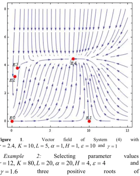
Example 1: Choose parameter values

10

,1

,1

,

5

,

10

,

4

.

2

=

=

=

=

=

=

K

L

α

H

ε

r

and γ =1 .

These values lead to Case 3(ii) where

0

,

0

<

>

a

b

and

a

2

>

3

b

(12) resulting in

0833 . 2 75 . 8 9 )

(_{x =x}3_{− x}2_{+ x−}

P .

The cubic polynomial

P

(

x

)

has three positive roots at

6890

.

0

,

3813

.

0

2

1

=

x

=

x

, and x3=7.9297 with local

maximum P(x1)=0.17504 for x1 =0.5336 and local minimum

P

(

x

2

)

=

0

−

59

.

8417

for

x

2

=

5

.

4664

. Since the

cubic P(x) has three positive roots the system has three equilibrium points in the population quadrant. It is routine to classify the three non-trivial equilibrium points either by calculating the eigenvalues or using the trace/determinant classification of the Jacobian at each point. These non-trivial equilibrium points are E2(0.3813,3.1887) ,

) 7743 . 3 , 6890 . 0 (

3

E and

E

4

(

7

.

9297

,

4

.

4370

)

and are

[image:4.595.315.555.453.754.2]

classified respectively as an attracting spiral point, a saddle and an attracting node. Using Mathematica [17], these saddles and the stable equilibrium points are shown in the vector field as depicted in Figure (1).

Figure 1. Vector field of System (4) with

10 , 1 , 1 , 5 , 10 , 4 .

2 = = = = =

= K L α H ε

r and γ =₁

Example 2: Selecting parameter values

4

,

4

,

20

,

20

,

80

,

12

=

=

=

=

=

=

K

L

α

H

ε

r

and

6

.

1

=

3 2

76

1280

67

.

4266

)

(

x

x

x

x

P

=

−

+

−

+

are attained, but

with corresponding points of different character. The roots of this polynomial are x₁=4.4312,x₂=17.9614andx₃=53.6074. Consequently there are three non-trivial equilibrium points

) 7785 . 4 , 4312 . 4 (

2

E , E3(17.9614,10.2184) and )

4031 . 11 , 6074 . 53 (

4

[image:5.595.311.553.72.319.2]

E . They are classified as an unstable node, a saddle point and an attracting spiral point respectively as shown in Figure (2).

Figure 2. Vector field of System (4) with

4 , 4 , 20 , 20 , 80 ,

12 = = = = =

= K L α H ε

r and γ=1.6

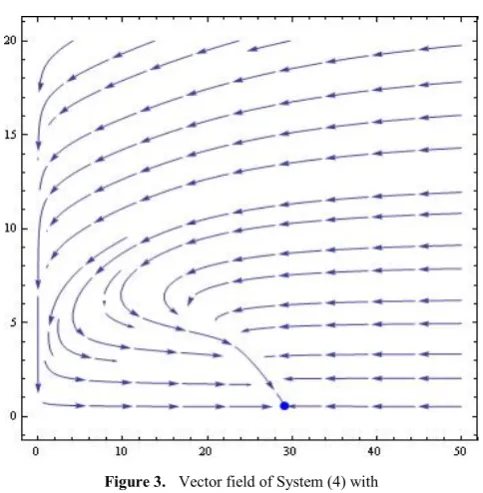
Example 3: For this example choose the parameter values

2 , 2 . 6 , 20 , 20 , 30 ,

12 = = = = =

= K L

α

H

ε

r and

6

.

1

=

γ

.

This produces the cubic polynomial 3

2

8

.

23

14

44960

)

(

x

x

x

x

P

=

−

+

−

+

.

There is a single root

x

₁

=

29

.

155

giving rise to the attracting node (29.155, 0.5975) as shown in Figure (3).

Figure 3. Vector field of System (4) with

2 , 2 . 6 , 20 , 20 , 30 ,

12 = = = = =

= K L α H ε

r and γ =1.6

Remark. There are two cases where the cubic

P

(

x

)

has three roots but one root is repeated. These cases are: (1) when there is a local maximum that just touches the

x

−

axis at say

x

₁ and the third root

x

₂ is larger than

x

₁; and (2) when there is a local minimum just touching the

x

−

axis at say

x

₂ and the third root is

x

₁ which is smaller than

x

₂. In both these cases, the critical value determined by the double root is unstable and trajectories are numerically sensitive near this point. The reader can verify Case 1 using

parameter values

10

,

10

,

25

,

026758

.

5

,

19

,

4

.

2

=

=

=

=

=

=

K

L

α

H

ε

r

and γ =0.011350 and Case 2 using

1

,

15

,

2

,

85454

.

7

,

22

,

1

=

=

=

=

=

=

K

L

α

H

ε

r

and

0173611 .

0

=

γ

.

In summary: No general conclusion may be drawn regarding the number or nature of the equilibrium points under Case 3(ii) where

b

>

0

,

a

<

0

and

a

2

_>

3

b

_.

Translated in terms of parameters present in System (4), this means that, for the FGH model, no conclusion can be drawn if

(

)

3 ( ( ) ) 0

and 0 ) ) ( ( , 0

2_{− − − >}

> − − <

−

ε γ ε α

ε γ ε α

Hr L

K H−K

Hr L

K K

H ₍₁₃₎

E0 E1

E2

E3 E4

0

20

40

60

80

[image:5.595.61.296.110.474.2]

The exclusion of this possibility is reflected in the following theorem regarding the uniqueness of the equilibrium point in the population quadrant of the FGH model.

Theorem 1: System (4) possesses a unique equilibrium point in the population quadrant at

₀

<

x

*

<

K

_and

(

1

/

)(

)

/

α

*

_r

_x

_K

_H

_x

y

=

−

+

if

(i)

L

α

(

ε

−

γ

)

−

Hr

ε

≤

0

,

or

(ii)

H

2

+

HK

+

K

2

−

(

3

KL

α

/

r

ε

)

(

ε

−

γ

))

≤

0

, or (iii)

L

α

(

ε

−

γ

)

−

Hr

ε

>

0

and

H

−

K

>

0

Proof

If either of Case1, 2 or 3(i) is satisfied, then there exists a unique positive root to the Cubic (9) and by implication System (4) possesses a unique

x

* in the population quadrant. Furthermore, since

0

<

x

*

<

K

, it follows that

(

1

/

)(

)

/

α

*

_r

_x

_K

_H

_x

y

=

−

+

is also positive and unique. Consequently

(

x

*

,

y

*

)

is a unique equilibrium point in the population quadrant of System (4).

With reference to Theorem 1 the FGH model with parameter values ensuring a unique equilibrium in the population quadrant, is in fact robust and results in system stability, yielding equilibrium values which lead to either limit cycles or attracting spiral points.

4. Conclusions

The FGH model supports the feature that the solutions are bounded from the onset by the carrying capacity of the prey and the population saturation of the predator. This makes applying Poincaré-Bendixson theory possible as long as the equilibrium point in the population quadrant is unique. Indeed, there is a wide variation of all parameters values for which the FGH model is robust and results in a stable system having equilibrium values which lead to either limit cycles or attracting spiral points. More details on this behaviour is given in a follow-up article as the FGH model is tested against a classification of Gunawardena [7] for perturbation caused by changes in initial values, parameter values or the dynamical functions. This test demonstrated that the FGH model does not require precise parameter values and can tolerate significant perturbation whilst the number and type of equilibrium points stay the same.

Remark: Although the FGH model can tolerate significant perturbations, the numerical methods require adaptive approaches based on iterative techniques. The numerical estimate of the solutions is not straightforward. For example, if epsilon in (1) is very small then adaptive mesh generations are necessary. Please refer to ([2],[3],[4],[5],[6],[7]) for more detail on numerical methods which requires adaptive mesh generations with the error analysis on these meshes.

REFERENCES

[1] B.S. Attili, S.F. Mallak, Existence of limit cycles in a predator-prey system with a functional response of the form Arctan(ax). Communications in Mathematical Analysis. 1. pp. 33-40, 2006.

[2] P. Das and V. Mehrmann, Numerical solution of singularly perturbed convection-diffusion- reaction problems with two small parameters, BIT Numerical Mathematics, 56, 51-76, 2016.

[3] P. Das, Comparison of a priori and a posteriori meshes for singularly perturbed nonlinear parameterized problems, Journal of Computational and Applied Mathematics, 290, 16-25, 2015.

[4] P. Das and S. Natesan, Adaptive mesh generation for singularly perturbed fourth order ordinary differential equations, International Journal of Computer Mathematics, 92(3), 562-578, 2015.

[5] P. Das and S. Natesan, Optimal error estimate using mesh equidistribution technique for singularly perturbed system of reaction-diffusion boundary value problems, Applied Mathematics and Computation, 249, 265-277, 2014.

[6] P. Das and S. Natesan, Higher order parameter uniform convergent schemes for Robin type reactiondiffusion problems using adaptively generated grid, International Journal of Computational Methods, 9(4), 2012, doi:10.1142/S0219876212500521.

[7] P. Das and S. Natesan, A uniformly convergent hybrid scheme for singularly perturbed system of reaction-diffusion Robin type boundary value problems, Journal of Applied Mathematics and Computing, 41(1-2), 447-471, 2013. [8] J. Gunawardena , Models in systems biology: the parameter

problem and the meanings of robustness. Elements of Computational Systems Biology. John Wiley and sons, New York, 2010.

[9] X. Huang, Y. Wang , L. ZhuOne and three limit cycles in a cubic predator-prey system. Mathematical Methods in the Applied Sciences. 30. pp. 501-511, 2007.

[10]X.C. Huang, L. Zhu, Limit cycles in a general Kolmogorov model. Nonlinear Analysis. 60. pp. 1393 – 1414, 2004. [11]R.E. Kooji, A. Zegeling, A predator-prey model with Ivlev's

functional response. Journal of Mathematical Analysis and Applications. 198. pp. 473-489, 1996.

[12]A.J. Lotka, Elements of Physical Biology. Williams & Wilkins, Baltimore, 1925.

[13]P.A. Schmidt, L.D. Mech Wolf Pack Size and Food Acquisition. Am. Nat. 150(4) pp. 513-517, 1997.

[14]M. Rosenzweig, R. MacArthur, Graphical representation and stability conditions of predator-prey interaction, American Naturalist 97: 209-223, 1963.

[16]J. Vandermeer, How Populations Grow: The Exponential and Logistic Equations. Nature Education Knowledge 3(10):15, 2010.

[17]S. Wolfram, The Mathematica Book, 3rd ed. Wolfram Media /Cambridge University Press, New York, 1999.

[18]D.G. Zill, M.R. Cullen, Advanced Engineering Mathematics. Second ed. Massachusetts: Jones and Bartlett Publishers, 2000.