Statistical Features-ANN Recognizer for Bivariate
Process Mean Shift Pattern Recognition
Ibrahim Masood
1, Adnan Hassan
21Faculty of Mechanical and Manufacturing Engineering, Universiti Tun Hussein Onn Malaysia 86400 Parit Raja, Batu Pahat, Johor, Malaysia
Email: [email protected]
2Faculty of Mechanical Engineering, Universiti Teknologi Malaysia 81310 UTM Skudai, Johor, Malaysia
Email: [email protected]
Abstract - Artificial neural network (ANN)-based recognizers have been developed for monitoring and diagnosis bivariate process mean shift in multivariate statistical process control (MSPC). They have better average run lengths (ARLs) performance in monitoring process mean shifts and gave an useful diagnosis information compared to the traditional
MSPC schemes such as T2, multivariate cumulative sum
(MCUSUM) and multivariate exponentially weighted moving average (MEWMA). The existing recognizers are raw data-based, whereby raw data input representation were applied into ANN. This approach required in a large network size, more computational effort and training time consuming. In this paper, the statistical features input representation was investigated, whereby the raw data were transformed into exponentially weighted moving average, multiplication of mean with standard deviation and multiplication of mean with mean-square value. The statistical features-ANN recognizer resulted in smaller network size, fast training time, better ARLs for monitoring process mean shifts and comparable recognition accuracy for diagnosing the source variable(s) compared to the raw data-ANN recognizer.
Keywords-Artificial neural network; bivariate process; statistical features input representation; multivariate quality control; statistical features
I. INTRODUCTION
Multivariate quality control (MQC) has become an important area of research in-line with their increasing application in manufacturing industries. Numerous multivariate statistical process control (MSPC) schemes have been proposed for monitoring and diagnosing multivariate process mean shift. A review on traditional MSPC charts and multivariate statistical techniques can be found in [1]. The traditional MSPC charts refer to the T2, multivariate cumulative sum (MCUSUM) and multivariate exponentially weighted moving average (MEWMA), whereas the multivariate statistical techniques refer to the principal component analysis (PCA) and partial least square (PLS). They described the most significant methods for the interpretation of an out-of-control signal. The review is useful for the new researchers towards improving MQC system.
In the related study, there has been an increasing trend focusing on pattern recognition of bivariate process
variables or quality characteristics. Rule-based expert
system, artificial neural network (ANN)-based recognizers and decision tree learning have been applied in developing the bivariate process pattern recognition (BPPR) schemes [2]; [3]; [4]; [5]; [6]; [7]; [8]; [9]; [10].
The rule-based expert system applied into the BPPR has been reported in [2]; [3]. Abnormality in the source variable(s) was represented by common causable patterns, i.e., upward and downward shifts, upward and downward trends, cyclic, systematic and mixture patterns.
The integrated MSPC-ANN schemes have been developed for similar purpose [5]; [6]; [7]. MSPC charts (T2
and T2-variance control charts) were applied for monitoring
process mean shift, whereas ANN-based recognizers were applied for diagnosing the source variable(s) that responsible for the mean shift. Abnormality in the source variable(s) was represented by upward and downward shift patterns.
In recent years, pure ANN-based recognizers have been proposed [4]; [8]; [10]. Investigation on a generalized-ANN model, namely novelty detector can be found in [4]. Then, a modular-ANN model that comprises two sequential modules has been investigated [8]. Module-1 contents a generalized-ANN for monitoring and diagnosing bivariate process mean shifts, whereas module-2 contents four specialized-ANNs for identifying the mean shift magnitudes. More recently, an ensemble-ANN model with ‘discrete particle swarm optimization’ (DPSOEN) algorithm has been studied [10].
The decision tree learning has also been applied into the BPPR [9]. Abnormality in the source variable(s) was focused on upward and downward shift patterns.
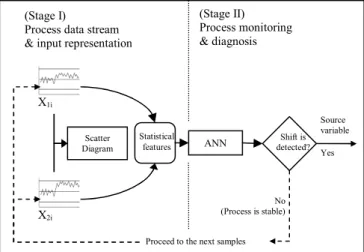
II. STATISTICAL FEATURES-ANNRECOGNIZER Statistical features-ANN recognizer comprises two main stages, i.e., (i) process data streams and input representation, and (ii) process monitoring and diagnosis, as shown in Figure 1. In first stage, data streams of two dependent process variables were plotted on a scatter diagram to yield bivariate shift patterns. Based on the scatter diagram, data streams were then transformed into statistical features input representation into an ANN. This will be described further in Section IV.
In second stage, an ANN model was applied for monitoring and diagnosing the bivariate process mean shifts through pattern recognition method. Monitoring refers to the identification of process status, i.e., either in a statistically stable state or in a statistically unstable state. Diagnosis refers to the identification of the source variable(s) that responsible for the statistically unstable state. In monitoring aspect, an ANN recognizer should able to detect a statistically unstable process as quickly as possible with small ARL1 (small Type II errors) and should able to leave a statistically stable process running as long as possible with large ARL0 (small Type I error). In diagnosis aspect, an ANN recognizer should able to identify the source variable(s) with high RA.
Figure 1. Conceptual diagram for the statistical features-ANN recognizer.
III. MODELING OF BIVARIATE PROCESS
Bivariate process is the simplest case in MQC when only two process variables are being monitored dependently. Let X1i = (X1-1,…, X1-24) and X2i = (X2-1,…, X2-24) represent data streams for process variable 1 and process variable 2 based on observation window - 24 samples. Observation windows for both variables start with samples ith = (1,…, 24). Then, it is followed with (ith +1), (ith + 2), …., and so on.
In a statistically stable state, samples for both process variables are identically and independently distributed (i.i.d.) with zero mean (μ0 = 0) and unity standard deviation (σ0 = 1). They yield random patterns when separately plotted on the Shewhart control charts and yield an ellipse pattern when plotted on a scatter diagram. Scatter diagram can indicate a measure of degree of linear relationship between two variables, i.e., cross correlation of data. Increasing the values of correlation will result in slim ellipses, as shown in Figure 2.
X1
X2
2 1 0 -1 -2 -3 3
2
1
0
-1
-2
-3
-4
Correlation = 0.0
X1
X2
3 2 1 0 -1 -2 -3 -4 3
2
1
0
-1
-2
-3
Correlation = 0.4
X1
X2
3 2 1 0 -1 -2 -3 -4 4
3
2
1
0
-1
-2
-3
Correlation = 0.8
Figure 2. Bivariate stable process patterns with different data correlation.
Disturbance from assignable causes may suddenly or gradually deteriorates data streams X1i and/or X2i into a statistically unstable state. Initially, the structure of an unstable pattern was vague or ‘partially developed’. Then, the pattern structure would be more obvious into ‘fully developed pattern’, as illustrated in Figure 3.
Figure 3. Process changes in upward-shift pattern.
Generally, the occurrence of assignable causes over X1i and/or X2i can be identified by common causable patterns such as upward and downward shifts, upward and downward trends, cyclic, systematic, and mixture. This study concerns on upward-shift and downward-shift patterns. Seven possible conditions of bivariate process mean shifts with positive correlation were considered, as summarized in Table I.
• Normal (0,0): Both X1i and X2i are stable
• Up-shift (1,0): X1i in upward-shift, X2i remain stable
• Up-shift (0,1): X2i in upward-shift, X1i remain stable
• Up-shift (1,1): Both X1i and X2i in upward-shifts
• Down-shift (1,0): X1i in downward-shift, X2i remain stable
• Down-shift (0,1): X2i in downward-shift, X1i remain stable
• Down-shift (1,1): Both X1i and X2i in downward-shifts TABLE I
CLASSIFICATION FOR THE BIVARIATE PROCESS MEAN SHIFT X2i
X1i
Scatter Diagram (Stage I)
Process data stream & input representation
Shift is detected?
Proceed to the next samples No (Process is stable)
ANN
(Stage II) Process monitoring & diagnosis
Statistical features
A. Data Generator
Ideally, observation samples should be tapped from real process environment. However, due to extensive demands for training and testing samples, Monte-Carlo simulation approach was applied for generating synthetic data as the following:
Step 1:
Generate random normal variates for process variable 1 (n1)
and process variable 2 (n2), which are identically and
independently distributed within [-3, +3]. b = 1/3 is a baseline noise level or random noise. In MATLAB, r is coded as ‘randn (row number, column number)’.
n1 = b. r1 (1)
n2 = b. r2 (2)
Step 2:
Generate random data series for process variable 1 (Y1) with
mean (μ1) and standard deviation (σ1), e.g. (μ1, σ1) = (50, 2).
Y1 = μ1 + ( n1 . σ1) (3)
Step 3:
Generate random data series for process variable 2 (Y2)
dependent to process variable 1 (Y1). μ2 and σ2 are the
values of mean and standard deviation for process variable 2, e.g. (μ2, σ2) = (100, 5). Based on Polar Method [11], random
normal variates are scaled into bivariate dependent variable by including correlation coefficient (ρ) into the basic equation (3).
Y2 = μ2 + [ n1 . ρ + n2(√ 1 - ρ2 ) ] σ2 (4)
Step 4:
Compute means and standard deviations for Y1 and Y2
respectively using the large sets of random data series, e.g. 1000. These values represent a statistically stable process means and standard deviations for process variable 1 (μ01,
σ01) and process variable 2 (μ02, σ02).
Step 5:
Transform random data series into normal or shift patterns to mimic real observation samples (X1, X2). h is the
magnitude of mean shift in standard deviation of stable process (σ01, σ02). h = 0 for normal patterns and h ≠ 0 for
shift patterns.
X1 = h1(σ01/ σ1) + Y1 (5) X2 = h2 (σ02/ σ2) + Y2 (6)
Step 6:
Rescale pattern data series into a standardize range, i.e. approximately [-3, 3].
Z1 = ( Y1 - μ01 ) / σ01 (7)
Z2 = ( Y2 - μ02 ) / σ02 (8)
Standardized samples (Z) follow N (0, R), where R is a general correlation matrix.
R = [(1 ρ) (ρ 1)] with unity variances (σ2
1 = σ22 = 1) and
covariance (σ12 = ρ).
B. Reference Patterns
In monitoring bivariate process, patterns should be able to indicate concurrent effects from process mean shifts and cross correlation of data. Unique structures of Shewhart control chart patterns provide useful meaning about process variation in mean shift in the source variable(s) but unable to indicate changes in data correlation. On the other hand, T2-statistic patterns consider multivariate process mean shift and data correlation but unable to diagnose the source variable(s).
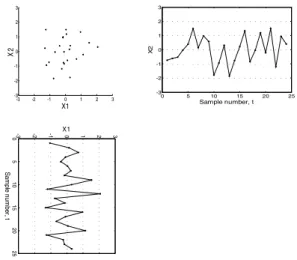
Distribution of samples of bivariate process using scatter diagram has been reported in [7]. The structures of bivariate process patterns can be differentiated and interpreted effectively in-line with changes in mean shifts in the source variable(s) and changes in data correlation. Pattern properties can be represented numerically either in the form of standardized samples (raw data) or features. Figure 4 shows a scatter diagram that comprises 24 standardized samples of process variable 1 (X1) and process variable 2 (X2)
yields a bivariate stable process pattern (Normal (0, 0)) with an approximately ellipse shape and zero-point center position.
-3 -2 -1 0 1 2 3
-3 -2 -1 0 1 2 3
X1
X2
0 5 10 15 20 25
-3 -2 -1 0 1 2 3
Sample number, t
X2
Figure 4. Bivariate process pattern for Normal (0, 0) condition.
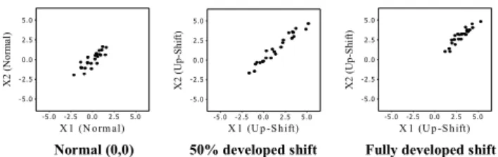
Bivariate process patterns that attributed to the similar assignable causes would share common structure and properties that are identifiable and recognizable. Process mean shift could be identified when the center position was shifted away from zero-point. Increment in data correlation could be identified with slim ellipse shapes. Figure 5 and Figure 6 show bivariate process patterns for Normal (0,0), 50% developed Up-shift (1,1) and fully developed Up-shift (1,1) conditions based on mean shift 3 standard deviations.
X 1 (N orm al)
X2
(N
orm
al
)
5.0 2.5 0 .0 -2 .5 -5 .0 5.0
2.5
0.0
-2.5
-5.0
X 1 (U p -S hift)
X
2 (
U
p-S
hif
t)
5.0 2 .5 0 .0 -2 .5 -5 .0 5.0
2.5
0.0
-2.5
-5.0
X 1 (Up-S hift)
X2
(
U
p-S
hif
t)
5 .0 2 .5 0.0 -2 .5 -5.0 5.0
2.5
0.0
-2.5
-5.0
Normal (0,0) 50% developed shift Fully developed shift
Figure 5. Patterns for Normal (0, 0), 50% developed up-shift (1,1) and fully developed up-shift (1,1) - low data correlation
0
5
10
15
20
25
-3 -2 -1 0 1 2 3
S
a
mp
le
n
u
mb
e
r, t
X 1 (N orm al)
X2
(
N
or
m
al
)
5.0 2 .5 0 .0 -2 .5 -5 .0 5.0
2.5
0.0
-2.5
-5.0
X 1 (U p -S hift)
X2
(
U
p-Sh
if
t)
5.0 2 .5 0 .0 -2 .5 -5 .0 5.0
2.5
0.0
-2.5
-5.0
X 1 (U p -S hift)
X2
(
U
p-S
hi
ft
)
5.0 2 .5 0 .0 -2 .5 -5 .0 5.0
2.5
0.0
-2.5
-5.0
Normal (0,0) 50% developed shift Fully developed shift
Figure 6. Patterns for Normal (0, 0), 50% developed up-shift(1,1) and fully developed up-shift (1,1) - high data correlation
IV. INPUT REPRESENTATION
Input representation provides a strong influence on an ANN performance. Besides raw data, feature-based approach has been reported in [13]; [14]; [15]; [16]. Ref. [13]
used minimal set of statistical features that consisted of
mean, standard deviation, skewness, mean-square value, autocorrelation and last value of cumulative sum. Ref. [14] firstly proposed nine shape features. The improved sets of shape features were then proposed in [15]; [16]. The proposed feature sets were reported to have better recognition accuracy of ANN compared to raw data. An improved set of statistical features was proposed for this study.
A. Raw Data Input Representation
Raw data input representation contained 24 consecutive standardized samples data sets (Zi). Each data set comprised two standardized samples for variable 1 and variable 2 (Zi_P1,
Zi_P2 ). Noted that i is the number of samples (1, 2, … , 24).
Variable 1 and variable 2 were denoted as P1 and P2 respectively. It can be written in series as [ Z1_1 , Z1_2 , Z2_1 , Z2_2 , Z3_1 , Z3_2 , … , Z24_1 , Z24_2 ]. Each patterns were represented by 48 = (24 x 2) inputs.
B. Statistical Features Input Representation
Statistical features input representation contained six features data sets, i.e. the last values of EWMA with constant parameter, λ = 0.10, 0.15, 0.20 and 0.25 (EWMA010, EWMA015, EWMA020, EWMA025), multiplication of mean with standard deviation (MSD), and multiplication of mean with mean-square value (MMS). Each data set contained statistical features for both variables, e.g. EWMA010-1 and EWMA010-2. It can be written in series as [ EWMA025-1 , EWMA020-1 , EWMA015-1 , EWMA010-1 , MSD1 , MMS1 , EWMA025-2 , EWMA020-2 , EWMA015-2 , EWMA010-2 , MSD2 , MMS2 ]. These values were used for strengthening pattern properties and improving discrimination capability between small shift and large shift patterns. Each pattern were represented by 12 = (6 x 2) inputs, four times smaller than the raw data input representation.
The EWMA can be viewed as a weighted average of all past and current observation samples, i.e., the historical data is considered in monitoring process mean shifts. It can be obtained by linear transforming the non-standardized observation samples (Xi) using the following equation:
EWMAi = λ Xi + (1 – λ) EWMAi-1 (9)
In this study, the standardized samples (Zi) were used instead of Xi. Therefore, equation (9) becomes:
EWMAi = λ Zi + (1 – λ) EWMAi-1 (10)
where, 0 < λ≤ 1 is a constant parameter and i is the number of samples (1, 2, … , 24). The starting EWMA value at first sample (EWMA0) represents the process target (μ0), so that
it is set as zero.
The multiplication of mean with standard deviation (MSD) feature is used to magnify the mean vectors for improving discrimination capability among the patterns.
For variable 1, MSD1 = μ1 x σ1 (11) For variable 2, MSD2 = μ2 x σ2 (12)
μ1 and μ2 are the means of Xi_p1 and Xi_p2 , whereas σ1 and
σ2 are the standard deviations of Xi_p1 and Xi_p2 respectively. The multiplication of mean and mean square values (MMS) feature also aims to magnify the mean vectors.
For variable 1, MMS1 = μ1 x (μ1)2 (13) For variable 2, MMS2 = μ2 x (μ2)2 (14) (μ1)2and (μ1)2 are the mean-square values of Xi_p1 and Xi_p2.
V. ANNRECOGNIZER DESIGN
Multilayer perceptron (MLP) model trained with back-propagation (BPN) algorithm was selected. MLP model basically comprises an input layer, one or more hidden layer(s) and an output layer. The number of layers and neurons in each layer could influence an ANN performance. Thus, it should be properly selected during the design stage. As a general guideline, an ANN size should be as small as possible to allow for efficient computation [12].
Figure 7 compares the network structures for three-layer MLP models. The number of input representation determined the number of input neurons. Statistical features input representation yields only 12 neurons compared to the raw data that needs 48 neurons. The output layer contains seven neurons, which was determined according to the number of pattern classes. One hidden layer with 24 neurons was selected based on preliminary experiment. Such experiments revealed that initially, the training results improved in-line with the increment in the number of neurons. Once the neurons exceeded 24, further increment of the neurons did not improve the training results but there were circumstances that indicated the training became worst. This shows that a huge or too many neurons could burden the MLP network computationally and could damage it generalization capability, thus, increases the training time.
(a) Raw data-ANN (b) Statistical features-ANN Figure 7. Network architectures for three layer MLP models.
Input Hidden Output layer (12) (24) (7 neurons)
..
..
..
.. ..
..
O1
O2
O3
O4
O5
O6
O7 Input Hidden Output layer
(48) (24) (7 neurons)
..
..
..
.. ..
..
O1
O2
O3
O4
O5
O6
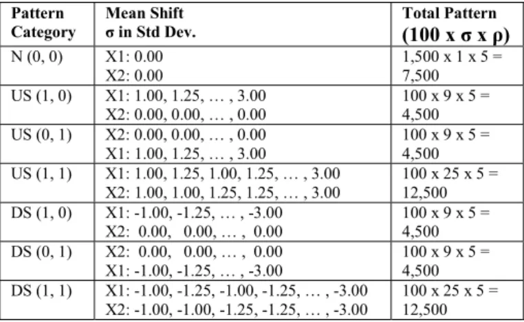
VI. ANNRECOGNIZER TRAINING AND TESTING Partially developed patterns with 50% shift area were applied for training the ANN recognizer. Each pattern comprised 24 standardized samples (Zi): samples 1 to 12 in
random normal, whereas samples 13 to 24 in shift. The cross correlation coefficient (ρ) was set to (0.1, 0.3, 0.5, 0.7 and 0.9) for all patterns.Detail parameters were summarized in Table II.
TABLE II
PARAMETERS FOR THE TRAINING PATTERNS
Pattern Category
Mean Shift
σ in Std Dev.
Total Pattern
(100 x σ x ρ) N (0, 0) X1: 0.00
X2: 0.00
1,500 x 1 x 5 = 7,500 US (1, 0) X1: 1.00, 1.25, … , 3.00
X2: 0.00, 0.00, … , 0.00
100 x 9 x 5 = 4,500 US (0, 1) X2: 0.00, 0.00, … , 0.00
X1: 1.00, 1.25, … , 3.00
100 x 9 x 5 = 4,500 US (1, 1) X1: 1.00, 1.25, 1.00, 1.25, … , 3.00
X2: 1.00, 1.00, 1.25, 1.25, … , 3.00
100 x 25 x 5 = 12,500 DS (1, 0) X1: -1.00, -1.25, … , -3.00
X2: 0.00, 0.00, … , 0.00 100 x 9 x 5 = 4,500 DS (0, 1) X2: 0.00, 0.00, … , 0.00
X1: -1.00, -1.25, … , -3.00
100 x 9 x 5 = 4,500 DS (1, 1) X1: -1.00, -1.25, -1.00, -1.25, … , -3.00
X2: -1.00, -1.00, -1.25, -1.25, … , -3.00
100 x 25 x 5 = 12,500
Input representation into ANN either as raw data or statistical features were rescaled/normalized to a compact range between [−1, 1]. The maximum and the minimum values for normalization were taken from the overall data of training patterns. This procedure has been implemented in other researches [13]; [15]; [16].
Based on BPN algorithm, ‘gradient decent with momentum and adaptive learning rate’ (traingdx) was used for training the MLP model. Learning rate and learning rate increment were set to 0.05 and 1.05, whereas maximum number of epochs and error goal were set to 1500 and 0.001 respectively. Network performance was based on mean square error (MSE). The hyperbolic tangent function was used for hidden layer to range the hidden output between [−1, 1] and sigmoid function was used for output layer to range the final output between [0, 1]. The training session was stopped either when the number of training epochs was met or the required MSE has been reached.
Dynamic patterns were applied for detail testing the ANN recognizers for implementation according to the on-line quality control situation. This approach has been addressed in [8].
VII.RESULTS AND DISCUSSION
The ANN performances for monitoring and diagnosing bivariate process mean shift were evaluated based on average run lengths (ARLs) and recognition accuracy (RA). Three thousand pattern examples were used in computing ARLs and RA for the specific magnitudes of mean shift and cross correlation. A good performance recognizer should have a large ARL0 (small Type I error) in identifying bivariate normal process, small ARL1 (small Type II error) in detecting bivariate process mean shifts and high RA in diagnosing the source variable(s). The ANN performances
were also compared with the traditional MSPC schemes, i.e., MC1 [17] and MEWMA [18] based on ARLs.
A. Average Run Lengths
The ARL1 results for the specific mean shift and the specific cross correlation as summarized in Table III were estimated by averaging the ARL1 on six shift pattern categories. The results were computed based on the correctly classified patterns. The results support the conclusion that the mean shift with larger magnitudes can be identified more quickly with shorter ARL1.
In identifying bivariate stable process, the statistical features-ANN recognizer has the largest ARL0 (smallest Type I error) compared to the raw data-ANN and the MSPC schemes. In detecting bivariate process mean shift, this recognizer provided smaller ARL1 (small Type II error) compared to the raw data-ANN (for large mean shifts) and the χ2 scheme. This ARL
1 results were close to the MC1 scheme.
Overall ARL performance indicating that the statistical features-ANN recognizer exhibits a strong ability for monitoring the bivariate process mean shift in on-line quality control situation.
TABLE III AVERAGE RUN LENGTHS
Mean Shift (σ in std dev)
Raw data-
ANN Statistical features-ANN χ
2
UCL=10.6
MC1
k= 0.50 h= 4.75
MEWMA
r = 0.10 h = 8.79
ρ = 0.3/0.8 ρ = 0.3 / 0.8 ρ = 0.0 ρ =0.0 ρ = 0.0 0.0 85 / NA 398 / NA 200 203 200
1.0 1.5 2.0 2.5 3.0
9.47 / 9.57 6.56 / 6.56 5.13 / 5.13 4.28 /4.29 3.69 /3.67
10.03 / 10.44 5.55 / 5.63 3.85 / 3.88 3.00 / 3.00 2.49 / 2.49
42.00 15.80 6.90 3.50 2.20
9.28 5.23 3.69 2.91 2.40
7.76 4.07 2.59 1.89 1.50
B. Recognition Accuracy
Table IV shows that the statistical features-ANN recognizer has better diagnosis capability compared to the raw data-ANN recognizer for up-shift (1,1) and down-shift (1,1) patterns, specifically for low data correlation. In this case, this recognizer also showed excellent recognition accuracy for high data correlation. On the other hand, the raw data-ANN recognizer provided better recognition accuracy compared to the statistical features-ANN in classifying the other shift patterns. Overall, both recognizers gave a comparable RA for low data correlation.
TABLE IV RECOGNITION ACCURACY
% Recognition Raw data-ANN ρ = 0.3 / 0.8
Statistical features-ANN ρ = 0.3 / 0.8
Normal (0,0) N/A N/A
Up-shift(1,0) 92.92 / 92.94 83.84 / 80.74
Up-shift(0,1) 89.24 / 88.28 92.14 / 91.14
Up-shift(1,1) 90.84 / 98.96 96.12 / 99.70
Downshift(1,0) 90.38 / 90.54 86.86 / 83.02
Downshift(0,1) 90.88 / 89.86 82.72 / 77.80
Downshift(1,1) 88.82 / 98.9 99.22 / 99.50
VIII.CONCLUSION
The statistical features-ANN recognizer is useful for implementation in MQC with smaller network size, better ARLs and comparable RA performances compared to the raw data-ANN recognizer. Small network resulted in fast training and allows for dealing with more complicated recognition, i.e., when more than two variables being monitored. The RA performance can be further improved with better input representation method, enhanced recognizer design and improved quality of training patterns.
REFERENCES
[1] S. Bersimis, S. Psarakis and J. Panaretos, “Multivariate statistical process control charts: an overview,” Quality and Reliability Engineering International, vol. 23, pp. 517−543, 2007.
[2] W. H. Chih and D. A. Rollier, “Diagnostic characteristics for bivariate pattern recognition scheme in SPC,” International Journal of Quality and Reliability Management, vol. 11, no. 1, pp. 53−66, 1994. [3] W. H. Chih and D. A. Rollier, “A methodology of pattern recognition
schemes for two variables in SPC,” International Journal of Quality and Reliability Management, vol. 12, no. 3, pp. 86−107, 1995. [4] F. Zorriassatine, J. D. T. Tannock and C. O’Brien, “Using novelty
detection to identify abnormalities caused by mean shifts in bivariate processes,” Computers and Industrial Engineering, vol. 44, pp. 385−408, 2003.
[5] L. H. Chen and T. Y. Wang, “Artificial neural networks to classify mean shifts from multivariate χ2 chart signals,” Computers and
Industrial Engineering, vol. 47, pp. 195−205, 2004.
[6] S. T. A. Niaki and B. Abbasi, “Fault diagnosis in multivariate control charts using artificial neural networks,” Quality and Reliability Engineering International, vol. 21, pp. 825−840, 2005.
[7] C. S. Cheng and H. P. Cheng, “Identifying the source of variance shifts in the multivariate process using neural networks and support
vector machines,” Expert Systems with Applications, vol. 35, pp. 198−206, 2008.
[8] R. S. Guh, “On-line identification and quantification of mean shifts in bivariate processes using a NN-based approach,” Quality and Reliability Engineering International, vol. 23, pp. 367−385, 2007. [9] R. S. Guh and Y. R. Shiue, “An-effective application of decision tree
learning for on-line detection of mean shifts in multivariate control charts,” Computers and Industrial Engineering, vol. 55, pp. 475−493, 2009.
[10] J. B. Yu and L. F. Xi, “A neural network ensemble-based model for on-line monitoring and diagnosis of out-of-control signals in multivariate manufacturing processes,” Expert Systems with Applications, vol. 36, pp. 909−921, 2009.
[11] A. M. Law and W. D. Kelton, Simulation modeling and Analysis, 3rd ed., Mc Graw-Hill, 2000.
[12] C. S. Cheng, “A neural network approach for the analysis of control chart patterns,” International Journal of Production Research, vol. 35, no. 3, pp. 667−697, 1997.
[13] A. Hassan, M. S. Nabi Baksh, M. A. Shaharoun and H. Jamaludin, “Improved SPC chart pattern recognition using statistical features,” International Journal of Production Research, vol. 41, no. 7, pp. 1587−1603, 2003.
[14] D. T. Pham and M. A. Wani, “Feature-based control chart pattern recognition,” International Journal of Production Research, vol. 35, no. 7, pp. 1875 − 1890, 1997.
[15] S. K. Gauri and S. Chakraborty, “Feature-based recognition of control chart patterns,” Computers and Industrial Engineering, vol. 51, pp. 726−742, 2006.
[16] S. K. Gauri and S. Chakraborty, “Improved recognition of control chart patterns using artificial neural networks,” International Journal of Advanced Manufacturing Technology, vol. 36, pp. 1191−1201, 2008.
[17] J. J. Pignatiello and G. C. Runger, “Comparisons of multivariate CUSUM charts,” Journal of Quality Technology, vol. 22, no. 3, pp. 173−186, 1990.