Lossless Compression of Grayscale Images Using Dynamic Arrays for Prediction and Applied to Higher Bitplanes

ISSN 2250-3153

Lossless Compression of Grayscale Images Using

Dynamic Arrays for Prediction and Applied to Higher

Bitplanes

Mayur Nandihalli

, Vishwanath Baligar

*

Dept. of Computer Science and Engineering B.V.Bhoomraddi College of Engineering and Technology Hubli, India **

Dept. of Computer Science and Engineering B.V.Bhoomraddi College of Engineering and Technology Hubli, India

Abstract- This paper presents a novel way of predicting pixel values of grayscale images using dynamic arrays. It is shown that the predicted values are always near to zero and this method does use a sign bit. Predicted values are compressed using bitplane method starting from 8th bitplane to 5th bitplane. The results shown are encouraging and comparable with the existing results.

Index Terms- RLE (run length encoding), bitplane, MSbs (Most Significant Bits).

I. INTRODUCTION

he discrete cosine transforms [1] in one dimension and two dimensions through which DCT coefficients were obtained from pixel values. These coefficients were further quantized and applied IDCT(Inverse) equation to reconstruct the original values. 6.4 % error was introduced between original and reconstructed values.

From 1990-1992, Pennebaker, Mitchell, Wallace and Zhang [1] conducted experiments on jpeg image compression. Color images were transformed from RGB to luminance/chrominance color space followed by down sampling of chrominance components which reduced the image to half of its original size. Pixels of each color components were organized into groups of 8x8 pixels. DCT was applied to these data units to obtain frequency components which were divided by a separate number called quantization coefficient and rounded to an integer. The quantized coefficients were encoded using run length encoding and Huffman coding. Very high compression ratios were obtained. In 1996, Weinberger et al. [1] found that a pixel can be predicted using its previous neighbors by assigning a probability distribution to them. Prediction error was also encoded.

In 1993, Howard and Vitter assigned variable size codes to each pixel based on the values of two of its previous neighbors [1] . The two neighbors with different intensities were selected based on the position of the current pixel. They assigned a variable size code based on the position of current pixel with respect to the neighbors selected. Wu in 1996 predicted a pixel using pixels all around it and also encoded the error values. Sayood and Anderson in 1992 found that image can be compressed by comparing each pixel P to a reference pixel which was one of its previously encoded immediate neighbors and encoded P in two parts prefix and suffix. A prefix which is the number of most significant bits of P that are identical to those of reference pixel and a suffix which is remaining least significant

bits of P. In 1998, Gilbert and Brodersen conducted experiments for lossless compression of discrete-tone images by scanning the image row by row and dividing the image into set of blocks of variable sizes namely copied blocks, solid fill blocks and punts. This method works by searching for a copy of current block and encoding the current block as width, height and location of copy block using Huffman codes.

This paper presents a new algorithm for lossless compression of grayscale images. The higher bitplanes are compressed using a new technique. This algorithm initializes arrays for every block of 8 X 8 pixels in a particular fashion. For every pixel in the block, a match is found in its respective array and storing the index value of the match in a new image file and later followed by dynamic shifts in the array. This new image file is named as encoded image. It also uses run length encoding for efficient compression. In section I and II, we explain compression of higher bitplanes and encoding of higher bitplanes respectively. In section III, the algorithm is explained in detail with an example. Finally in section IV, we conclude our study and summarize our results.

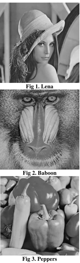
II. COMPRESSION OF HIGHER BITPLANES Higher bitplanes indicate 8th,7th,6th and 5th bitplanes which represent 8th,7th,6th and 5th bits of each pixel respectively. Higher bitplanes are compressed using run length encoding which are based on the raster scan of each bitplane. The degree of randomness of adjacent pixels is very low in higher bitplanes. Therefore, reasonable compression ratios are achieved in these bitplanes using run length encoding. The compressed versions of these bitplanes consists of numbers which represent the length of run of consecutive similar pixels. The figures Fig 1, Fig 2 and Fig 3 are the standard 512 x 512 images used for experimentation. The 8X8 matrix representing pixels is shown in

ISSN 2250-3153

Fig 1. Lena

Fig 2. Baboon

Fig 3. Peppers

A. Matrix Scan of Higher Bitplanes

Instead of going for raster scan, we prefer matrix scan which reduces the degree of randomness from pixel to pixel. The higher bitplanes are scanned as 8 x 8 matrices. The matrix scan reduces the degree of randomness of pixels within the matrix. Let us consider an example of matrix scan. A random 8 x 8 matrix of pixel values of fig 1. is shown in

TABLE I. These values range from 0 to 255. For the values in

TABLE I the match for each pixel is found in the array corresponding to its predicted value and index value of the match is fetched.

TABLE II shows the index values of the match found in arrays.

TABLE I

8 X 8 MATRIX REPRESENTING PIXEL VALUES 162 162 162 161 162 157 163 161 162 162 162 161 162 157 163 161 162 162 162 161 162 157 163 161 162 162 162 161 162 157 163 161 162 162 162 161 162 157 163 161 164 164 158 155 161 159 159 160 160 160 163 158 160 162 159 156 159 159 155 157 158 159 156 157

B. Assignment of Arrays

Each pixel value in

ISSN 2250-3153

C. Operation on Arrays

When pixels are matrix scanned, for each pixel except the pixels in the first column of the image, the predicted value is the previous pixel. For pixels in the first column, the predicted value is 128. In the original image of resolution 512 X 512, number of pixels in the first column are only 512. For these 512 pixels present in the first column of original image, the predicted value is 128. When a pixel is scanned, its respective predicted value’s array is taken into consideration followed by finding a match for current pixel in that array. When a match is found, the index value of match is considered for encoding. This index value plays a vital role in the compression of higher bitplanes. The index value of the match which ranges from 0 to 255 is stored in a new image file by considering the index as a pixel value. After storing the index value in a new file, the matched value in the array is inserted at the beginning of array from its original position, followed by successive shifts by one position till the original position of match is filled. If the match is found in the beginning of array, the values of array remain unchanged. In this manner, the values of arrays corresponding to the predicted value of each pixel keeps varying throughout the scan.

TABLE II

INDEX VALUES OF THE MATCH FOUND IN ARRAYS OF CORRESPONDING PREDICTED VALUES IN

BINARY FORM

68 0 0 0 1 2 9 12

0 2 0 2 0 2 0 0

0 2 0 2 0 2 0 0

0 2 0 2 0 2 0 0

0 2 0 2 0 2 0 0

72 0 11 5 12 3 0 2

66 0 6 9 5 5 6 5

65 2 7 5 3 4 2 2

III. ENCODING OF HIGHER BITPLANES Once the whole image is matrix scanned, for each pixel, the index value of its match is stored in a new image file as shown in

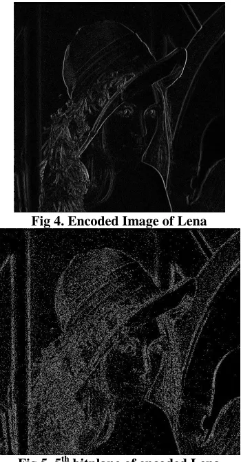
TABLE II. The encoded image file consists of index values which represent each pixel of the original image. In the encoded image file, the degree of randomness of higher bitplanes is too low. After all the pixels are scanned and encoded as index values, the adjacent most significant bits are highly correlated. The result of compression of higher bitplanes is shown in TABLE XIII. The encoded image of Fig 1. is shown in Fig 4. This encoded image consists of index values of the match as pixel values. The degree of randomness in the encoded image is comparatively low. Fig 5 to Fig 8 shows 5th, 6th, 7th and 8th bitplanes of encoded Lena respectively. These higher bitplanes are run length encoded to achieve very high compression ratios.

Fig 4. Encoded Image of Lena

ISSN 2250-3153

Fig 6. 6th bitplane of encoded Lena

Fig 7. 7th bitplane of encoded Lena Fig 8. 8th bitplane of encoded Lena

TABLE III VALUES OF ARRAY CORRESPONDING TO VALUE 0

0 255 1 254 2 253 3 252 - - - - - - 129 127

TABLE IV VALUES OF ARRAY CORRESPONDING TO VALUE 1

1 0 2 255 3 254 4 253 - - - - - - 130 128

TABLE V VALUES OF ARRAY CORRESPONDING TO VALUE 2

2 1 3 0 4 255 5 254 - - - - - - 131 129

TABLE VI VALUES OF ARRAY CORRESPONDING TO VALUE 3

3 2 4 1 5 0 6 255 - - - - - - 132 130

TABLE VII VALUES OF ARRAY CORRESPONDING TO VALUE 4

4 3 5 2 6 1 7 0 - - - - - - 133 131

TABLE VIII VALUES OF ARRAY CORRESPONDING TO VALUE 5

5 4 6 3 7 2 8 1 - - - - - - 134 132

TABLE IX VALUES OF ARRAY CORRESPONDINIG TO 128 AFTER SCANNING FIRST PIXEL

162 128 127 129 126 130 125 131 - - - - - - 1 255

TABLE X VALUES OF ARRAY CORRESPONDING TO 162 AFTER SCANNING SECOND PIXEL

ISSN 2250-3153

TABLE XI VALUES OF ARRAY CORRESPONDING TO 162 AFTER SCANNING FOURTH PIXEL

161 162 163 160 164 159 165 158 - - - - - - 35 33

TABLE XII VALUES OF ARRAY CORRESPONDING TO 161 AFTER SCANNING FIFTH PIXEL

162 161 160 159 163 158 164 157 - - - - - - 34 32

IV. OPERATIONS IN DETAIL

The tables numbered from TABLE III to TABLE VIII shows the initial values of arrays for 0 to 5 respectively. Same array initialization pattern is followed to assign all the arrays from 0 to 255. These arrays are initialized for every 8 X 8 matrix of pixels. To understand the operations in detail, let us take an example by considering the pixel values specified in

TABLE I. The first pixel is 162 and as it is the pixel of first column, its predicted value will be 128. Match for 162 should be found in the array corresponding to 128. After the match is found, the matched value is shifted to the first position followed by successive shifts to fill the matched position in the array. The values of array corresponding to 128 after scanning of first pixel is shown in TABLE IX. Second pixel in the matrix is 162 again. Its predicted value is the previous pixel i.e. 162. Match for 162 should be found in the array corresponding to 162. As the match for 162 in the array corresponding to 162 is found in the first position, no shifting takes place which is shown in TABLE X. Third pixel is again 162 and its predicted value is the previous pixel which is 162. So no changes are made in the array as the match is found in first position. Fourth pixel is 161 whose predicted value will be the previous pixel 162. Match for 161 in the array corresponding to 162 is found in the second position. TABLE XI shows the values of array after scanning fourth pixel. The next pixel in the matrix is 162 whose predicted value will be 161. The match for 162 is found in the array corresponding to 161 which is found at third position and shifting operations takes place. TABLE XII shows the values of array corresponding to 161 after scanning of fifth pixel. This process continues for all the pixels in every matrix. When a match is found, the index value of match is stored in an image file. This file consists of index values of all the matches which is shown in Fig 4. whose higher bitplanes are run length encoded.

TABLE XIII shows the results.

TABLE XIII

RESULTS OF COMPRESSION OF HIGHER BITPLANES

Image name

Bitplane number

Original size(bits)

Compress ed size(bits)

Compress ion ratio

Lena 8 262144 14177.60 18.49 : 1 7 262144 48455.45 5.41 : 1 6 262144 117553.36 2.23 : 1 5 262144 188592.80 1.39 : 1 Baboo

n

8 262144 8700.43 30.13 : 1 7 262144 25303.47 10.36 : 1 6 262144 123652.83 2.12 : 1 5 262144 211406.45 1.24 : 1 Pepper

s

8 262144 17000.25 15.42 : 1 7 262144 36308.03 7.22 : 1 6 262144 110144.53 2.38 : 1 5 262144 200109.92 1.31 : 1

TABLE XIV

OVERALL COMPRESSION RATIO OF HIGHER BITPLANES

Image name Original size (bits)

Compressed size (bits)

Compression ratio

ISSN 2250-3153

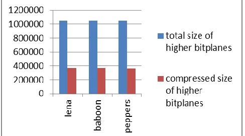
Fig 9. Final Results of Compression of Higher Bitplanes

Fig 9 shows graphical representation of compression of higher bitplanes of all the three sample images. TABLE XIV shows overall compression ratios of higher bitplanes for all the sample images.

TABLE XV

JPEG-LS COMPRESSION RATIO

Image name Original size (bits)

Compressed size (bits)

Compression ratio

Lena 2097152 1239016 1.69 : 1

Baboon 2097152 1212024 1.73 : 1 Peppers 2097152 1297968 1.61 : 1

V. CONCLUSION

In this paper we established a new method for lossless compression of higher bitplanes for grayscale images. This new method uses arrays whose index values are used to encode the image followed by shifting the array values dynamically after each match to obtain highly correlated adjacent values which is further encoded using run length encoding. This method results in efficient compression of higher bitplanes for grayscale images.

REFERENCES

[1] David Salomon, Data Compression, 3rd ed., New York: Springer-Verlag, 2005.

[2] Weinberger, M.J., G. Seroussi and G. Sapiro, “LOCO-I Low Complexity Context Based Lossless Image Compression Algorithm” in proceedings of data compression conference, 1996, pp. 140-149.

[3] Heath, F.G. “Origins of the Binary Code” Scientific American, 1972 August, 227(2): 76.

AUTHORS