Combination of Multiple Neural Networks to Solve
Travelling Salesman Problem using Genetic Algorithm
Anmol Aggarwal
Department of Information Technology, Bharati Vidyapeeth’s College of Engineering,
New Delhi, INDIA
Jasdeep Singh Bhalla
Department of Computer Science, Bharati Vidyapeeth’s College of Engineering,New Delhi, INDIA
ABSTRACT
In this paper, the already recognized NP Complete problem which is Travelling Salesman Problem which is also known as TSP, is addressed and its performance is analyzed. For a large and complex data set, a particular neural network is needed to focus on a particular component of the problem, after which combining of all the networks together is required. The basic ideology behind this multiple neural network arrangement is that, n-independently different neural networks are trained separately and then their respective outputs (generated independently) are combined together to form the resultant classifier. A new combining technique (for combining outputs of multiple neural networks into one) has been proposed and utilized for evidence blend in the simulation part of the method. Its performance is analyzed on the bases of simulation and it shows some notably enhanced outcomes.
Keywords
Travelling Salesman Problem, Artificial Intelligence, Multiple Neural Networks, Genetic Algorithm, ANNs, neural networks.
1.
INTRODUCTION
Recurrent developments have been done and are still going on in the improvement of intelligent and quick systems with high end methodologies; some have been stimulated by neural networks incorporating biological effects. Various formal methodologies have been proposed and deduced to solve these types of troubles and problems. Even though the acknowledged applications could be found in various presumed constrained environments, but nothing is sufficiently flexible to perform well exterior to its defined sphere. The Artificial Neural Networks provide such flexibility with massive parallelism and learning ability.
Modern digital computers can easily outperform humans in field of numeric computing, but they still cannot match the speed and accuracy in solving complex perceptual problems. To resolve this problem, an artificial neuron, which is a computer based form motivated by the innate neurons, has evolved. Learning in neural network is primarily a process of adjusting connection strengths at desired levels. Throughout the training process, adjustment of the input weights is done. This input weight showcases the connection’s strength (or bondness) towards the basic neuron unit in the subsequently next layer (consecutively next layer) of neural network. This association (connection) weight will manipulate and influence the input. Weights are referred as the coefficients with adaptive capabilities within the network which decides the strength of the inputted signal. Therefore, the preliminary weights for a in-process component could be
tailored in reaction to a variety of inputs and thereafter as per the network's own regulations meant for revision.
Fundamental advantages of Neural Networks:
They resemble to an actual real nervous system.
Corresponding association generates solutions to problems, where extensively multiple constraints ought to be fulfilled concurrently.
Rules are implicit in nature instead of explicit.
2.
ARTIFICIAL NEURAL NETWORKS
(ANNs)
Artificial neural network is often considered to as a simple neural network in computer science, is interpreted as a computational model representation based on neural networks (biological in nature). It constitutes a cluster of artificial neurons interconnected to each other which executes and processes the information by means of a simple connection-oriented approach for computational purpose. Within many scenarios, an Artificial Neural Network based on dynamic system (adaptive) that leads to various changes in its configuration on the basis of outer or inner information that transports through the network throughout the learning period.
2.1
Basic Topologies of Neural Network:
Fig. 1. Feedforward neural network
2.2
Distributed memory machine
: [image:2.595.83.255.376.533.2]Recurrent based neural network (frequently depicted as RNN) is referred to as a set of various neural networks which deals with associations linking units forming a directed loop or cycle. Thus, this produces a state which is internal state of the network allowing it to exhibit its dynamic (adaptive) behavior. Unlike the traditional feedforward based neural networks, the RNN (Recurrent Neural Network) exploit their interior memory which processes random input sequences in the system. Figure 2 depicts recurrent network.
Fig. 2. Recurrent network
2.3
Basic Working of Artificial Neural
Networks
A number of inputs are being received by the network. Each input is received by means of a bond which has an equivalent weight attached to it. Each neuron is linked with a corresponding threshold rate (or value). A sum of inputs (sum of input weights) is produced and its corresponding threshold value is removed to constitute the launch (activation or assigning) of the input. It may be noted here that negative weights can also be assigned as in [1]. This input activation is passed throughout a function which is based on input activation to yield the respective outcome [2].
Considerate functionalities of ANN’s are discussed below:
Dynamic behavior (Adaptability): It refers to the behavior of the network which is determined as per the input provided.
The network’s structure is altered in line with the data given.
Error (inaccuracy) forbearance
Real (genuine) time function
Analogous Information (or data) System
2.4
Concept of Multiple Networks
For a large and complex data set, a particular neural network is needed to focus on a definite part of the difficulty or problem and thereafter combining of the networks together is required. Thus, the concept of multiple neural networks comes into existence. A neural network generally trains with an information set and thereafter generates significant patterns, links and associations. Nevertheless, the network of fixed size doesn’t record the relations precisely. With the increase in number of layers it does not guarantee noteworthy improvements as per the sense of precision. The dataset (information set) is huge and is neither self-sufficient nor modular in complex problematic situations. Consequently, we can make a neural network to focus over a significant part of the problem and merge a number of networks together in combination.
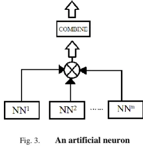
The fundamental proposal of multiple neural network (more than one neural network) system is typically meant to train n-independent networks (ANN) and after that, organize the units of input separately (or independently). As a final point, we sum up the results to get the resulting classifier which is acquired by the combination of these networks.
Fig. 3. An artificial neuron
2.5
Training Of Artificial Neural Networks
A neural network can be easily explained as a system that takes a set of inputs and yields the preferred set of outputs as an outcome or end result. A variety of different methods exist to set the strengths of the associations (or connections). Out of which, one approach is explicitly setting of the weights, using a pre known understanding. A different methodology is to ‘train’ the basic neural network by means of providing it training patterns and allowing it to modify its respective weights as per some pre defined learning. Now, categorizing of the profound learning situations is as follows:
[image:2.595.352.498.432.581.2]can be taken up by the internal system itself which constitutes the self-supervised neural network.
Unsupervised learning: In this, output unit is trained to give response to the clusters (group) of pattern present within the input units. Here, the system is constructed to determine statistically prominent characteristics of the inputs of population and give results. As compared to the case in supervised learning, there are no set of types (or categories) into which the links (or patterns) are to be considered. Therefore, the system must resort to its own demonstration of the input values.
Reinforcement Learning: Such kind of learning is taken as a middle type of the above specified kinds of learning. Generally, here in this specific case, learning module performs a few actions on the surroundings or the environment and receives a response feedback reply returned from the considered environment as an outcome. This learning module evaluates its action as good which in another sense means rewarding or bad which in another sense mean punishable, overall based on the environmental reaction.
3.
TRAVELLING SALESMAN
PROBLEM
The Travelling Salesman Problem frequently called as TSP is sort of problem which is generally used for computational mathematical problems intended at finding the shortest path that can be attained for paying a visit to each and every city mentioned on a given set of cities, attached with their acknowledged distances respectively. This is done for every city set, and get back to the preliminary position (or the initial point). A specified complete graph having n nodes is considered and these nodes, distinctly showcases the set of cities. The edge length shows the gap or distance between each pair of cities correspondingly. This TSP Problem has an objective of discovering mainly the proficient Hamiltonian Cycle or route a salesman can (or may) take (or follow) in traversing each of the n cities present. This type of problem is being recognized as a NP-Hard problem. A paramount resolution (or solution) for such kind of problem cannot be established on the basis of polynomial time. As, there is no permanent and traditionally existing efficient algorithm to estimate the finest explanation for this problem, thus, the time essential in such kind of solution would ascend exponentially along with enhancement of the size of the problem. In other words, time to resolve the problem in a situation like this would be a term that would enclose size of the problem n can be given to as an exponent value. To sum it up, we tried to trace an efficient and proficient solution nearby to the ideal scenario, which can be calculated in polynomial time. The TSP is proven to be an NP-hard problem based in the field of combinatorial based optimization mainly studied in operational research and other theoretical field of computer science. The major significant alternative to this would be to undertake the entire permutations and examine which one of them is significantly smaller using the brute force search. Therefore, the running time of this thought lies inside a polynomial factor of O (n!). Then the factorial of the total number of cities provided. One of the important and earliest applications of dynamic programming is this method that solves the problem in time O (n22n) [2].
This dynamic programming alternative asks for an exponential space. By using various inclusion–exclusion
methodologies, the problem can be solved in time within a polynomial factor of 2n and polynomial space. Enhancement of these time constraints seems to be a bit difficult. Therefore, this is not considered as a definite solution for this problem.
4.
USE OF GENETIC ALGORITHMS IN
SOLVING TRAVELLING SALESMEN
PROBLEM
Genetic algorithms are considered to be an optimization methodology. It is strongly based on the natural evolution of data. This concept works on the principle which is “survival of the fittest” and this proposal incorporated into a search algorithm providing a scheme of searching that does not require the exploration of every feasible explanation in the viable region to acquire a superior and effective result. In natural arena, the fittest individuals are most likely to survive and mate. Thus, the next generation would be fitter and healthier because they were generated from healthy parents.[4] This analogous idea is applied on to a problem by first guessing(or predicting) the solutions and then combining the fittest solutions mutually to craft a new generation of solutions which would be enhanced and superior than its preceding (or earlier) generation. Therefore, we tend to take in a random mutation element also to account (or consider) for the rare ‘mishap situation’ in nature.
4.1
Evolution of Genetic Algorithms
These genetic algorithms are comparatively fresh examples in the field of artificial intelligence, which work on the typical principles of natural assortment. The main theoretical concept for this was at first introduced by John Holland along with his scholar students in the mid 1970’s [3]. After that, regular enhancement in the performance and significance value of Genetic Algorithms has pushed them as one of the most significant algorithms of all times. These algorithms sufficiently work for many sorts of problem solving. In a sense, a genetic algorithm generally proves to be very sound on mixed and diverse (continuous and discrete) problems or complexities. These are less risky in order to get trapped at local level as compared to the gradient based search methods. Thereby, they are expensive in terms of computability and are considered as probabilistic algorithms in the field of computer science. A primary population called genome (famously known as chromosome) is generated in random fashion then succeeding populations (or generations), can be obtained using various genetic operators (typically which are as selection, crossover and mutation) to advance (or evolve) the preferred outcomes with a mindset to find the best case.
4.2
Genetic Algorithm
Step 1: Build the preliminary population of individual string for the provided problem randomly. Then produce a matrix representation of the cost of the path amongst the two of the considered cities.
Step 2: Every chromosome in the population is allocated fitness by fitness measure.
Where, x = total cost (string). The basis of selection is dependent on the sting’s value if it is close to the threshold rate (value).
Step 3: New off-spring population is built using two pre-existing chromosomes in the parent population by the use of crossover operator.
Step 4: If required, Mutation of the resultant off-springs is done.
NOTE: The fitness value of off-spring population is higher than the parents after the crossover.
Step 5: Repeat step 3 and 4 until we get an optimal solution to the problem.
[image:4.595.61.261.265.565.2]Flowchart below shows the procedure:
Fig. 4. Flowchart
5.
PROPOSED TECHNIQUE
In a multiple neural network system, n-independently different neural networks are trained separately and then their respective outputs which are generated independently are combined together to form a resultant. Here, we will put forward a novel combining technique (in order to combine the outputs of multiple neural networks into one)
5.1
Algorithm:
1) Division of the training sets into N pieces. (N = number of CPUs)
2) Then copy the Artificial Neural Network to N copies
3) After that, train each copy for 1...10 epochs (training cycle)
4) Finally combine the N networks to form N/2 networks by considering the weighted average in of the output unit of each network, weights depending upon the accuracy of each
network. Let the output from each copy is yj, than the overall
result y is defined as:
Where α is a set of weights considered.
5) Repeat until only one neural network is left.
6.
EXPERIMENTAL RESULTS
A simple test was done which indicates that the neural networks outcomes can be combined to obtain more acceptable and significant outcomes (results) for a large and multifaceted considered problem.
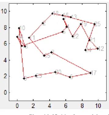
A multiple neural network combining technique is proposed in this paper, which differs amongst the count of neuron units in the hidden layer (intermediate layer), and the count of training procedures, each presuming an optimal (most favorable) way out for the travelling salesman problem along with the help of genetic algorithm. As shown below, the neural networks are being trained by utilizing the same training informational sets and subsequently their output values were observed. The training set iterations(procedures) are kept diverse for each and every neural network. Thus, a small set of interpretations and corresponding best path lengths are presented as graphical figures in the following section.
[image:4.595.317.496.436.625.2]Fig. 6. Plot with 50 cities (best path length=165.35)
Fig. 7. Plot with 100 cities (best path length=414.35)
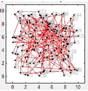
[image:5.595.56.234.290.472.2]Fig. 8. Plot with 150 cities (best path length=637.85)
[image:5.595.317.497.305.486.2]Fig. 9. Plot with 200 cities (best path length=909.35)
Fig. 10. Plot with 250 cities (best path length=1165.75)
[image:5.595.56.234.509.694.2] [image:5.595.317.498.525.698.2]Network was tested using Matlab (R2012b) software on three hundred different cities and their best path length responses were noted. Using this data, we measured their best paths through our proposed method which combined multiple neural networks along with genetic algorithm to resolve the already recognized travelling salesman problem (TSP).
7.
CONCLUSION
In this paper, authors have tried to resolve the basic Travelling Salesman Problem, by combining multiple neural networks to find the final output. Genetic Algorithm was used to train the artificial neural network. An algorithm for combining multiple neural networks was implemented. The results simulated were compared on the basis of best path length, suggested that combined mutual neural networks with the use of genetic algorithm along are apt for the problems which are complex in nature and for obtaining more precise results. As this field is not completely matured, a lot of work is still going on for solving complex problems with more perfection.
8.
FUTURE SCOPE
Further research may include intelligently dividing the whole network into various copies, depending on size and their effectiveness. The number of iterations the whole process should execute completely. Also more number of inputs can be taken, and thus, train the network to lessen the error probability and further enhance the effectiveness of the neural network
9.
REFERENCES
[1] Akshay Gupta, “Synthesis and Performance Analysis of Recurrent Fuzzy Multilayer Perceptron for Speech Recognition”, an IEEE International Conference on the Methods & Models in Computer Science, held in December 2010
[2] Akshay Gupta, Khushboo Aggarwal, “Multiple Neural Network Architecture for the Travelling Salesman Problem”, International Transactions on Applied
Sciences & Technology (ITAST) Volume :1 No 1 May,year 2011.
[3] Al-Dulaimi, Hamza A. Ali and Buthainah Fahran “Enhanced Traveling Salesman Problem Solvingby Genetic Algorithm Technique (TSPGA)”, The World Academy of Science,.. Engineering and Technology 14 2008.
[4] Hashem, S., B,. Schmeiser , "Approximating a function and its derivatives using MSE-optimal linear combinations of trained feedforward neural networks", The Proceedings of the Joint Conference on Neural Networks pg. 617–620
[5] David W. Opitz, Jude W. Shavlik, “A Genetic Algorithm Approach for Creating Neural-Network Ensembles”, Combining ANNs, A. Sharkey, Springer-Verlag, London, pp. 79-97, 1999.
[6] Jin H. Kim Sun Cho, , “Combining Multiple Neural Networks by Fuzzy Integral for Robust Classification” published in IEEE Transactions(System, Man and Cybernetics), Volume 25, No. 2, February 1995.
[7] Krishnan Chander, “Reservoir characterization using well log data with the aid of soft computing tools”, though it is an unpublished article.
[8] Durbin R. Rumelhart D. E.,Chauvin Y., “Backpropagation: The basic theory, architecture and application” Pgs 1 to 34. Lawrence Erlbaum, Hillsdale, NJ.
[9] Takayama K, Morva A, Obata Y, Nagai T, Fujikawa M, Hattori Y,., “Formula optimization of theophylline controlled-release tablet based on artificial neural networks”, Release; 68:175-186
[10] Simon Haykin, “Neural Networks, A Comprehensive Foundation”, Second Englewood Cliffs, NJ Prentice-Hall, 1999:156-254.