Fuzzy Hyperline Segment Neural Network Pattern Classifier with Different Distance Metrics

Fuzzy Hyperline Segment Neural Network Pattern

Classifier with Different Distance Metrics

K. S. Kadam

Assistant Professor,

Dept. of Electronics & Telecomm. Engineering KCT’s LGNSCOE, Nashik, (M. S.), India

S. B. Bagal

Associate Professor and Head, Dept. of Electronics & Telecomm. Engineering

KCT’s LGNSCOE, Nashik, (M. S.), India

ABSTRACT

The Fuzzy Hyperline Segment Neural Network (FHLSNN) pattern classifier utilizes fuzzy set as pattern classes in which each fuzzy set is a union of fuzzy set hyperline segments. The Euclidean distance metric is used to compute the distances to decide the degree of membership function. In this paper, the use of other various distance metrics such as Manhattan, Squared Euclidean, Canberra and Chebyshew distance metrics is proposed. The performance of FHLSNN pattern classifier is evaluated with various benchmark databases such as Glass, Wine, PID, and Iris data set and real handwritten database. The FHLSNN pattern classifier is evaluated for generalization performance under recognition rate, training time and testing time. From the result analysis, the performance of classifier is based on the distance metrics as well the database used is verified. This analysis will help to select a suitable distance metric for fuzzy neural network classifier for particular application.

General Terms

Pattern Recognition, Neural Network, and Distance metrics

Keywords

Fuzzy, Neural Networks, Fuzzy hyperline segment neural network (FHLSNN), Euclidean, Canberra, Chebyshew

1.

INTRODUCTION

In the recent years, hybrid systems that include the artificial neural network and fuzzy logic are popular for pattern recognition and classification. These systems are promising alternative to various conventional classification methods. An artificial neural network is network of interconnected neurons, inspired from the studies of the biological nervous system. The main characteristic of the neural network is the fact that these structures can learn with examples (training vectors, input and output samples of the system). The neural networks modify its internal structure and the weights of connections between its artificial neurons to make the mapping that represent the behavior of the modeled system. The advantages of the neural networks are learning capacity, generalization capacity and robustness in relation to disturbances. The fuzzy logic is an approach to computer science that mimics the way a human brain thinks and solves problems. The idea of fuzzy logic is to approximate human decision making using natural language terms instead of quantitative terms. The fuzzy neural networks (FNN) combine the strength of fuzzy logic and neural network.

There are several different implementations of fuzzy neural networks (FNN), and have been successfully applied to a variety of real world classification tasks in industry, business and science. Patrick K. Simpson proposed supervised learning

neural network classifier known as fuzzy min-max neural network that utilizes fuzzy sets as pattern classes where each fuzzy set is an aggregate of fuzzy set hyperboxes [1]. He has also proposed unsupervised fuzzy min-max clustering neural network in which clusters are implemented as fuzzy set using membership function with a hyperbox core that is constructed from a min point and a max point [2]. At the same time, Kwan and Cai have proposed four layer feed forward fuzzy neural network with unsupervised learning algorithm, which is used for character recognition [3]. G. Peter Zhang has presented a focused review of several important issues and recent developments of neural networks for classification problems. These include the posterior probability estimation, the link between neural and conventional classifiers, the relationship between learning and generalization in neural network classification, and issues to improve neural classifier performance [4]. In the sequel to Min-Max fuzzy neural network classifier, Kulkarni U. V. et al. proposed fuzzy hyperline segment clustering neural network (FHLSCNN). The FHLSCNN first creates hyperline segments by connecting adjacent patterns possibly falling in same cluster by using fuzzy membership criteria. Then clusters are formed by finding the centroids and bunching created HLSs that fall around the centroids [5]. Kulkarni U. V. et all have also presented fuzzy hyperline Segment neural network (FHLSNN) for rotation invariant handwritten character recognition that utilizes fuzzy set as pattern classes in which each fuzzy set is a union of fuzzy set hyperline segments [6]. In FHLSNN, the Euclidean distance metric is used to compute the distances

and for the calculation of membership function. A.

Vadivel, A. K. Majumdar, and Shamik Sural compare the performance of various distance metrics in the content-based image retrieval applications [7].

In this paper, the use of various distance metrics to compute the distances and for the calculation of membership

function of FHLSNN is proposed also the performance of these distance metrics with various benchmark databases is analysed. The performance of FHLSNN pattern classifier is also evaluated for real handwritten character recognition. The FHLSNN pattern classifier is evaluated for recognition rate, generalization, training time and testing time with different distance metric and different datasets. The objective of this paper is to check the suitability of distance metric for fuzzy neural network classifier for particular application.

description of data sets and discussions on the results are presented in Section 5. Finally, the conclusion is given in section 6.

2.

TOPOLOGY OF

FHLSNN

The architecture of FHLSNN consists of four layers as shown in Figure 1. In this architecture first, second, third and fourth layer are denoted as and respectively. The first layer accepts an input pattern and consists of n processing elements, one for each dimension of the pattern. The layer

consists of m processing nodes that are constructed during training. There are two connections from each to each

node. Each connection represents an end point for that particular hyperline segment. One end point is stored in matrix V and the other end point in matrix W. Each node represents hyperline segment fuzzy set and is characterized by the membership function.

( , , …… , )

Fig 1: Fuzzy Hyperline Segment Neural Network

Let represents the hth input

pattern, is the one end point of

hyperline segment and is the

other end point of . Then the membership function of the jth node is defined as

(1)

in which and the distances and are defined as

(2)

(3)

(4)

and is the three parameter ramp threshold function defined as

(5)

The layer gives soft decision and output of kth node represents the degree to which the input pattern belongs to the class . The binary weights assigned to the connections between and layers are stored in the matrix U. The values assigned to these connections are defined as

for and (6) where is the jth _{node and d}

k is the kth node.

The transfer function of each node perform the union of the appropriate (of same class) hyperline segment fuzzy values which is described as

for (7)

Each node delivers nonfuzzy output descried as

where , for k=1 to p. (8)

3.

LEARNING ALGORITHM OF

FHLSNN

The supervised FHLSNN learning algorithm for creating HLSs in the hyperspace consists of following steps.

Step 1: Initialization. To initialize HLS start with first pattern in the database, as

(9) Step 2: Creation of hyperline segments. The maximum length of HLS is bounded by the parameter θ, where

which is a user defined value and depends on the dimension of feature vector. The extension criterion that has to be met before HLS can extend to include is

. (10)

Let the set of pattern is R, where . Given the hth training pair find all the HLSs belonging to the class . After this following cases are carried out for possible inclusion of the input pattern . Case 1: By using membership function, find out whether the pattern falls on any one of the exiting HLSs. If falls on any of the HLS then it is included. Therefore, in the training process all the remaining steps are skipped and training is continued with the next training pair.

Case 2: If the input pattern falls on any one of the hyperlines passing through the two end points of HLS, then extend the HLS to include the pattern. Suppose is that hyperline segment with end points and then are calculated using equation (2), (3), and (4). Subsequently algorithm executes sub-step (i) if , else the sub-step (ii). Otherwise the Case 3 is considered.

Layer

Matrix Layer

Layer

(i) Test whether the point falls on the HLS formed by the points and using equation (1) and if verified then include the pattern by extending as

and (11) (ii) Test whether the point falls on the hyperline segment formed by the points and and if verified, then include the pattern by extending as

_{and . (12)}

Case 3: If HLS is a point i.e. , then extend it to include the pattern , if extension criteria is satisfied as described by equation (11).

Case 4: If the pattern is not included by any of the HLSs then create a new HLS as

_{. (13)}

Step 3: Intersection test. The learning algorithm allows intersection of HLSs from the same class and eliminates the intersection between HLSs from separate classes. Intersection test is carried out as soon as the HLS is either extended by Case 2, Case 3 or created in Case 4.

Let and

represent two end points of the extended or created HLS and

are the end points of the HLS of other class. The equation of hyperline passing through and is

(14)

and the equation of the hyperline passing through and is

(15)

where , are the constants and are the variables. The

equations (14) and (15) leads to set of n simultaneous equations which are described as

(16) For

The values of and can be calculated by solving any two simultaneous equations. If remaining n-2 equations are satisfied with the calculated values of and then two hyperlines are intersecting and the points of intersection is

(17) The point of intersection , if falls on both hyperlines segments then these HLSs are also intersect. This can be verified by the equation (1) and eliminated by contraction of appropriate HLS.

Step 4: Removing intersection. Depending on the cases, if extension of HLS produces an intersection then it is removed by restoring the end point as , and point is restored as, . Create a new HLS to include as in equation (13).

If Case 4 creates intersection then it is removed by restoring the end points of previous HLS of other class as

and . (18)

4.

DISTANCE METRICS

To compute the three distances l, l1, l2 given by equation (2) to (4), various distance metrics can be used. In this paper, five distance metrics are used to implement classifier. In pattern recognition studies the importance goes to finding out the relevance between patterns falling in n-dimensional pattern space. To find out the relevance between the patterns the characteristic distance between them is important to find out. So the characteristics distance between the patterns plays important role to decide the classification criterion. If this characteristics distance has changed then the classification criteria may be changed. To describe aforementioned concept, the example of Euclidean distance and the Manhattan distance is given here. Euclidean distance is the direct straight line geometrical distance between the two points as shown in Figure 2. This distance can be easily calculated by equation (19).

Y

Euclidean Distance

X

Fig 2: Concept of Euclidean Distance.

While Manhattan distance is the city block distance between two points as shown in Figure 3. Refer equation (20).

Y

City Block Distance (Manhattan)

X

Fig 3: Concept of Manhattan Distance.

Considering above example it is clear that though the two points A and B remains at same position in pattern space but the distance between them has changed if the metric or method to calculate distance is changed.

Hence in pattern classification studies it is important to know how the pattern classification result, i.e. recognition rate changes with various distance metrics. However it will be very interesting to know which distance metric is suitable for particular distance metric. The results presented in this paper may help to decide the distance metric choice for particular application. Consider the points

and , then the distance between these

4.1

Euclidean Distance

(19)

4.2

Manhattan Distance or City Block

Distance

(20)

4.3

Chebyshew Distance or Maximum

Metric

(21)

4.4

Canberra Distance

(22)

4.5

Square Euclidean distance

It is not the distance metrics, as it does not satisfy the triangle inequality. But it is very easy to calculate this distance mathematically.

(23)

5.

EXPERIMENTS AND RESULTS

This is implemented using MATLAB R2013a and ran on Intel core i3 2328M, 2.2GHz PC. To evaluate the different capabilities of a pattern classifier, five benchmark data sets from the UCI machine learning repository [9] and the real handwritten character database is selected. A description of each data set is as follows.

1) The Glass data set: This data set contains 214 samples, each with nine continuous features, from six classes. Six classes are building window float processesd, building window non-float processesd, vehical windows non-float processed, containers, tablewares and headlamps glass. Nine features are Refractive index, Sodium, Magnesium, Aluminium, Silicon, Potassium, Calcium, Barrium and Iron. 2) The Wine data set: This data set is another example of multiple classes with continuous features. This data set contains 178 samples, each with 13 continuous features. Features are alcohol, malic, ash, alcalinity, magnesium, phenols, flavanoids, non-flavanoids, proanthocyanins, color, hue, 10D280/0D315 of diluted wines, and proline.

3) The PID data set: This data set consists of 768 cases with eight features from two classes (diabetic and healthy). A total of 268 cases (35%) are from patients diagnosed as diabetic and the remaining as healthy. The samples from data set are overlapping each other, making a challenging classification problem.

4) The Iris data set: This data set contains 150 samples, each with four continuous features (sepal length, sepal width, petal length, and petal width), from three classes (Iris setosa, Iris versicolor, and Iris virginica). This data set is an example of a small data set with a small number of features. One class is linearly separable from the other two classes, but the other two classes are not linearly separable from each other. 5) Sonar Data set: This data set is the example of high-dimensional data set which contains 208 samples; all patterns have 60 input features. The data set contains 111 patterns from mine samples (metal cylinders) (class 1) and 97 patterns from rocks samples (class 2).

6) Real handwritten character database: This database consists of consists of 1000 Devanagari a numeral character. Ten numerals from one hundred writers are scanned and stored in

BMP format. After moment normalization [10], the rotation invariant ring-data features defined by Ueda and Nakamura [11] and extended by Chiu and Tseng [12], are extracted from the character by setting ring width to two. The extracted ring-data vector is a 16-dimensional feature vector.

Set 1 and Set 2 are obtained from all the original five databases described above. Set 1 consists of half of randomly selected patterns from each class given for training and remaining half of patterns of each class given for testing. Set 2 is reverse generalization for Set 1 i.e. patterns which are given for training in Set 1 are given for testing in Set 2 and vice-versa. 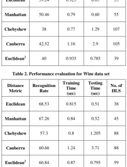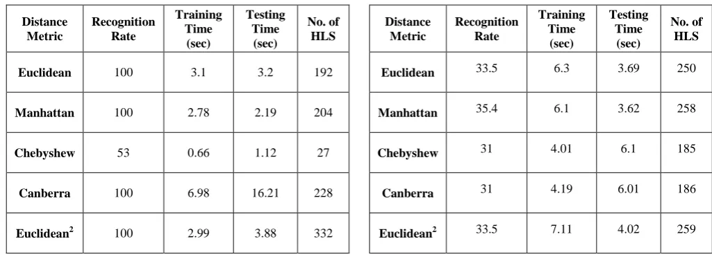The results mentioned in the observation tables from Table 1 to Table 6 are for generalization ability of classifiers and it is the average result of Set 1 and Set 2.

As patterns given for learning of classifier are totally different for the patterns given for testing hence 100% recognition cannot be expected since testing is for generalization ability of classifiers. The performance of FHLSNN is evaluated for recognition rate in percentage, training time in seconds and testing time in seconds with different distance metric mentioned in section IV for different datasets. Table 1 to Table 6 shows the performance evaluation of FHLSNN for Glass data, Wine data, PID data, Iris data Sonar data and Real world handwritten characters data respectively.

Table 1. Performance evaluation for Glass data set

Distance Metric

Recognition Rate

Training Time

(sec)

Testing Time

(sec)

No. of HLS

Euclidean 39.24 0.925 0.63 55

Manhattan 50.46 0.79 0.60 55

Chebyshew 38 0.77 1.29 107

Canberra 42.52 1.16 2.9 105

Euclidean2 40 0.935 0.785 39

Table 2. Performance evaluation for Wine data set

Distance Metric

Recognition Rate

Training Time

(sec)

Testing Time

(sec)

No. of HLS

Euclidean 68.53 0.815 0.51 38

Manhattan 67.26 0.84 0.52 45

Chebyshew 57.3 0.8 1.205 88

Canberra 60.66 1.24 3.71 88

Table 3. Performance evaluation for PID data set

Distance Metric

Recognition Rate

Training Time

(sec)

Testing Time

(sec)

No. of HLS

Euclidean 100 3.1 3.2 192

Manhattan 100 2.78 2.19 204

Chebyshew 53 0.66 1.12 27

Canberra 100 6.98 16.21 228

Euclidean2 100 2.99 3.88 332

Table 4. Performance evaluation for Iris data set

Distance Metric

Recognition Rate

Training Time

(sec)

Testing Time

(sec)

No. of HLS

Euclidean 94.66 0.48 0.54 39

Manhattan 93.33 0.51 0.52 34

Chebyshew 34.66 0.71 0.92 75

Canberra 95.33 0.96 1.1 42

Euclidean2 94.66 0.75 0.74 35

Table 5. Performance evaluation for Sonar data Set

Distance Metric

Recognition Rate

Training Time

(sec)

Testing Time

(sec)

No. of HLS

Euclidean 54.80 8.89 0.90 88

Manhattan 33.33 0.63 1.16 139

Chebyshew 99.66 4.59 2.17 71

Canberra 33.33 6.92 28 138

Euclidean2 55 9.76 1.33 115

Table 5. Performance evaluation for handwritten data Set

Distance Metric

Recognition Rate

Training Time

(sec)

Testing Time

(sec)

No. of HLS

Euclidean 33.5 6.3 3.69 250

Manhattan 35.4 6.1 3.62 258

Chebyshew 31 4.01 6.1 185

Canberra 31 4.19 6.01 186

Euclidean2 33.5 7.11 4.02 259

From the results summarized in Table 1 to Table 5, then it is observed that all the distance metrics have different performance in terms of recognition rate, training time and testing time. This variation in the performance is observed against same dataset and on same classifier, but with different distance metric. Distance metric changes the relevance or correlation value in the n-dimensional pattern space. On the same benchmark above experimentation can justify the effect on classification by deploying different distance metrics. The Canberra distance metric gives lower recognition rate and more training and testing time for all the data sets, but it surprisingly gives a good recognition rate for Iris data set. This classifier requires more training and testing time to classify PID dataset for Canberra distance. The Manhattan distance also gives a comparable performance for the entire data base in term of recognition rate, training and testing time. The Chebyshew distance or Maximum metric is does not gives satisfactory result for the entire data base. Thus the results shows that the performance of selected classifier is based on the distance metrics as well the database used.

6.

CONCLUSION

7.

REFERENCES

[1] P. K. Simpson, “Fuzzy min–max neural networks—Part 1: Classification,” IEEE Trans. Neural Networks., vol. 3, no. 5, pp. 776–786, Sep. 1992.

[2] P. K. Simpson, “Fuzzy min–max neural networks—Part 2: Clustering,” IEEE Trans. Fuzzy systems, vol. 1, no. 1, pp. 32–45, Feb. 1993.

[3] Kwan H. K. and Yaling Cai, “A fuzzy neural network and its applications to pattern recognition,” IEEE Trans. Fuzzy Systems, vol. 2, no. 3, pp 185-192, Aug. 1994. [4] G. Peter Zhang, “Neural Network for Classification: A

Survey,” IEEE Trans. System, Man and Cybernetics, C, Applications and Review, vol.30, no. 4, pp. 451-462, Nov 2000.

[5] U. V. Kulkarni, T. R. Sontakke, and A. B. Kulkarni, “Fuzzy hyperline segment clustering neural network,” Electronics Letters, IEE, vol. 37, no. 5, pp. 301–303, March. 2001.

[6] U. V. Kulkarni, T. R. Sontakke, and G. D. Randale, “Fuzzy hyperline segment neural for rotation invariant handwritten recognition,” published in int. joint conf. on neural networks: IJCCNN’01 held in Washington DC, USA, July 2001, pp. 2918–2923.

[7] A. Vadivel, A. K. Majumdar, and S. Sural, “Performance comparison of distance metrics in content-based Image retrieval applications,” in Proc. 6th International Conf. Information Technology, Bhubaneswar, India, Dec. 22-25, 2003, pp. 159-164.

[8] Johnson, R.A., and D.W. Wichern, 1998. Applied multivariate Statistical Analysis. New Jersey: Prentice Hall. pp. 226-235.

[9] P. M. Murphy and D. W. Aha, UCI Repository of Machine Learning Databases, (Machine-Readable Data Repository). Irvine, CA: Dept. Inf. Comput. Sci., Univ.California, 1995.

[10] Perantonis S.J. and P.J.G. Lisboa, “Translation, rotation and scale invariant pattern recognition by high-order neural networks and moment classifiers”, IEEE Trans. Neural networks, Vol. 3, No. 2, 1992, pp. 241-251. [11] Udea K. and Y. Nakamura, “Automatic verification of

seal impression pattern”, In: Proc. 9th internat. Conf. on pattern recognition.Vo1. 2, 1984, pp. 1019-1021. [12] Hung-Pin Chiu and Din-Chang Tseng, “Invariant