A Hybrid Reasoning Model for “Whole and Part” Cardinal Direction Relations

Kor, A and Bennett, B (2013) A Hybrid Reasoning Model for “Whole and Part” Cardinal Direction

Rela-tions. Advances in Artificial Intelligence. ISSN 1687-7489 DOI: https://doi.org/10.1155/2013/205261

Link to Leeds Beckett Repository record:

http://eprints.leedsbeckett.ac.uk/709/

Document Version:

Article

Creative Commons: Attribution 3.0

The aim of the Leeds Beckett Repository is to provide open access to our research, as required by

funder policies and permitted by publishers and copyright law.

The Leeds Beckett repository holds a wide range of publications, each of which has been

checked for copyright and the relevant embargo period has been applied by the Research Services

team.

We operate on a standard take-down policy.

If you are the author or publisher of an output

and you would like it removed from the repository, please

contact us

and we will investigate on a

case-by-case basis.

Research Article

A Hybrid Reasoning Model for ‘‘Whole and Part’’ Cardinal

Direction Relations

Ah-Lian Kor

and Brandon Bennett

1_{Arts Environment and Technology Faculty, Leeds Metropolitan University, Headingley Campus, Leeds LS6 3QS, UK} 2_{School of Computing, University of Leeds, Leeds LS2 9JT, UK}

Correspondence should be addressed to Ah-Lian Kor; [email protected]

Received 8 May 2012; Accepted 24 September 2012

Academic Editor: Ian Mitchell

Copyright © 2013 A.-L. Kor and B. Bennett. This is an open access article distributed under the Creative Commons Attribution License, which permits unrestricted use, distribution, and reproduction in any medium, provided the original work is properly cited.

We have shown how the ninetilesin the projection-based model for cardinal directions can be partitioned into sets based on

horizontal and vertical constraints (calledHorizontal and Vertical Constraints Model) in our previous papers (Kor and Bennett,

2003 and 2010). In order to come up with an expressive hybrid model for direction relations between two-dimensional single-piece regions (without holes), we integrate the well-known RCC-8 model with the above-mentioned model. From this expressive

hybrid model, we derive 8 basic binary relations and 13 feasible as well as jointly exhaustive relations for thex- andy-directions,

respectively. Based on these basic binary relations, we derive two separate8 × 8composition tables for both the expressive and

weak direction relations. We introduce a formula that can be used for the computation of the composition of expressive and weak direction relations between “whole or part” regions. Lastly, we also show how the expressive hybrid model can be used to make several existential inferences that are not possible for existing models.

1. Introduction

Relative positions of regions in large-scale spaces, and partic-ularly in the geographic domain, are often described by rela-tions referring to cardinal direcrela-tions. These relarela-tions specify the direction from one region to another in terms of the familiar compass bearings: north, south, east, and west. The intermediate directions northwest, northeast, southwest, and southeast are also often used. Some models for reasoning with

cardinal directions are the cone-shaped [1, 2],

projection-based models (ibid), and direction matrix [3–5].

Papadias and Theodoridis [6] describe topological and

direction relations between regions using their minimum bounding rectangles (MBRs). However, the language used is not expressive enough to describe direction relations. Additionally, the MBR technique yields erroneous outcome

when involving regions that are not rectangular in shape [4]

Some work has been done on hybrid direction models. Escrig

and Toledo [7] and Clementini et al. [8] integrated qualitative

orientation and distance to obtain positional information.

Isli [9] combined Frank’s [1, 2] cardinal direction relations

model and Freksa’s [10] orientation model to facilitate a more

expressive reasoning mechanism. Sharma and Flewelling

[11] infer spatial relations from integrated topological and

cardinal direction relations. Liu and colleagues [12] have

developed reasoning algorithms which combine RCC-8 [13]

for topological relations (discussed inSection 4) and the

car-dinal direction calculus (CDC [3–5], discussed inSection 2)

for direction relations. Li and colleagues’ work [14, 15]

focuses on the development and evaluation of an efficient reasoning mechanism for RCC-8 and RA (Rectangle Algebra,

and further explanation can be found in [16,17]) which is

employed to solve the satisfiability problem of these two joint constraint networks.

Typically, composition tables are used to infer spatial relations between objects. They have been employed to make

different inferences about cardinal directions relations [3,19–

North

South

East West

N NE NW

E W

S

SW SE

Position of an observer

Figure 1: Cone-shaped direction model with 4 or 8 partitions (ibid).

EQ North

South North

South

Ea

st

Ea

st

We

st

We

st

Two separate sets of

half-planes

Two integrated sets of

half-planes NE NW

SE SW

(Frank, 1992 and 1996)

(Frank, 1992 and 1996)

(Ligozat, 1998)

Point B

Figure 2: Cardinal directions defined by half-planes.

can lead to tractable computation of inferences [25]. In this

paper, we have developed an expressive hybrid model for direction relations. We will describe the binary relations in

the model and define“whole and part”relations. Based on this

model, we derive two8 × 8composition tables forexpressive

and weakdirection relations. This is followed by introducing a

formula which could be used to compute bothexpressive and

weakdirection relations for“whole and part”regions. Finally,

we will demonstrate how the model could be used to make several types of existential inferences.

2. Cardinal Direction Models

Frank [1, 2] defines cardinal directions as cones which

are related to the angular direction between an observer’s position (in the form of a point) and a destination point. The cone-shaped cardinal direction model could have 4, 8,

or more partitions (look atFigure 1).

Frank defines the four major cardinal directions (north, south, east, and west) as pair-wise opposites and half planes. When the two sets of half planes are combined, it yields four intermediate cardinal directions (northeast, northwest,

southeast, and southwest) which are depicted in Figure 2.

Ligozat [21] applies the model to points in a two-dimensional

space. Thus, the referent object,Point B, will be given the four

major directions. However, the relations between two objects will be denoted by one of the following basic relations: N, S, E, W, NE, NW, SE, SW, or EQ.

Region

NE( )

SE( )

SW( ) S( )

W( )

N( )

E( ) O( )

NW(𝑎

𝑎

𝑎 𝑎

𝑎 𝑎

𝑎 𝑎

𝑎

𝑎 )

Figure 3: Cardinal directions defined by tiles for extended objects

[1,2].

Frank [1,2] extends the half-planes to tiles for regions (as

shown inFigure 3). In this projection-based model, the plane

of an arbitrary single-piece regionais partitioned into nine

tiles, North-West, NW(a); North, N(a); North-East, NE(a); South-West, SW(a); South, S(a); South-East, SE(a); West, W(a); Neutral Zone, O(a); East, E(a). According to Frank, the O tile is considered a neutral zone, because in this tile, the relative cardinal direction between two regions cannot be determined due to their proximity.

Frank compares and contrasts reasoning with the cone-shaped and the projection-based models for cardinal direc-tions. The reasoning capability for both the systems is limited and weak though they do not differ substantially in their reasoning outcomes. In order to create a more expressive

rea-soning model, Isli [26] integrates the Frank’s cone-shaped and

projection-based models to facilitate reasoning about relative position of points of the 2-dimensional space. This hybrid model is well suited for applications of large-scale high-level vision, such as, for example, satellite-like surveillance of a geographic area.

The cardinal direction calculus (CDC) [3–5] is a very

expressive qualitative calculus for directional information of

extended objects. A direction relation matrix (DRM) in (1)

is used to represent direction relations between connected

plane regions. Liu and colleagues [27, 28] have shown that

consistency checking of complete networks of basic CDC constraints is tractable, while reasoning with the CDC in gen-eral is NP hard. However, if some constraints are unspecified, then consistency checking of incomplete networks of basic CDC constraints is intractable.

The cardinal direction of a target object (regionb) to a

referent object (regiona) as shown inFigure 4is described by

recording those tiles covered by the target object. According

to Goyal and Egenhofer [4], a 3 × 3 matrix is employed

to register the intersections between the target object and

the tiles of the referent object (see (1)). The elements in

the direction-relation matrix correspond to the tiles of the

referent object, regiona(inFigure 4).

In (1), the symbol 0 represents empty tile while ¬0

represents nonempty tile. These are used to describe cardinal

directions at a coarse granularity level. InFigure 4, region𝑏

Region_𝑏

Region

NE( )

SE( )

SW( ) S( )

W( )

N( )

E( ) O( )

NW(𝑎

𝑎

𝑎 𝑎

𝑎 𝑎

𝑎 𝑎

𝑎

𝑎 )

Figure 4: Nine tiles with regions𝑎(as the referent object) and𝑏(as

the target object) [4,5].

𝑋max(𝑎)

Horizontal set Vertical set

𝑋min(𝑎)

𝑌min(𝑎

𝑎

)

𝑌max(𝑎)

Figure 5: Horizontal and vertical sets oftilesfora.

tiles are considered nonempty while the rest are considered

empty (as shown in (1)).

Goyal and Egenhofer [5] extend the direction relation

matrix, so that it will be more expressive. Instead of using the empty and nonempty notations, it registers how much (in terms of proportion) the target region occupies each tile

(see (2)). The expressive direction relation matrix in (2) has

6 elements of zero and three nonzero elements which sum up to 1.0. If the matrix has only one nonzero element then it

is known as asingle element direction relation matrixwhile

a matrix with more than one nonzero element is called a multielement direction relation matrix(ibid).

Coarse direction relation matrix [4]:

dir_𝑅𝑅(𝑎, 𝑏) = (

NW(𝑎) ∩ 𝑏 N(𝑎) ∩ 𝑏 NE(𝑎) ∩ 𝑏 W(𝑎) ∩ 𝑏 O(𝑎) ∩ 𝑏 E(𝑎) ∩ 𝑏 SW(𝑎) ∩ 𝑏 S(𝑎) ∩ 𝑏 SE(𝑎) ∩ 𝑏

) ,

dir_𝑅𝑅(𝑎, 𝑏) = (

0 ¬0 ¬0 0 0 ¬0 0 0 0) .

(1)

dir_𝑅𝑅(𝑎, 𝑏)

= ((

(

area(NW(𝑎) ∩ 𝑏)

area of𝑏

area(N(𝑎) ∩ 𝑏)

area of𝑏

area(NE(𝑎) ∩ 𝑏)

area of𝑏 area(W(𝑎) ∩ 𝑏)

area of𝑏

area(O(𝑎) ∩ 𝑏)

area of𝑏

area(E(𝑎) ∩ 𝑏)

area of𝑏 area(SW(𝑎) ∩ 𝑏)

area of𝑏

area(S(𝑎) ∩ 𝑏)

area of𝑏

area(SE(𝑎) ∩ 𝑏)

area of𝑏

) )

) ,

dir_𝑅𝑅(𝑎, 𝑏) = (

0 0.05 0.45 0 0 0.50 0 0 0 ) .

(2)

3. Horizontal and Vertical Constraints Model

Every region has a minimal bounding box with specific

minimum and maximum𝑥(and𝑦) values. The boundaries

of the minimal bounding box of a region𝑎are depicted in

Figure 5. The set of boundaries of the minimal bounding

box for region𝑎could be represented as{𝑋_min(𝑎),𝑋_max(𝑎),

𝑌_min(𝑎),𝑌_max(𝑎)}, and these values will be employed to define

each tile.

The definition of the nine tiles in terms of the boundaries of the minimal bounding box is listed as below. Note, in this paper, all the tiles are regarded as mutually exclusive. Thus neighboring tiles cannot share common boundaries:

(i) N(𝑎) ≡ {⟨𝑥, 𝑦⟩|𝑋_min(𝑎)≤ 𝑥<𝑋_max(𝑎) ∧ 𝑦≥𝑌_max(𝑎)},

(ii) NE(𝑎) ≡ {⟨𝑥, 𝑦⟩|𝑥≥𝑋_max(𝑎)∧𝑦≥𝑌_max(𝑎)},

(iii) NW(𝑎) ≡ {⟨𝑥, 𝑦⟩|𝑥<𝑋_min(𝑎)∧𝑦≥𝑌_max(𝑎)},

(iv) S(𝑎) ≡ {⟨𝑥, 𝑦⟩|𝑋_min(𝑎)≤𝑥<𝑋_max(𝑎)∧𝑦<𝑌_min(𝑎)},

(v) SE(𝑎) ≡ {⟨𝑥, 𝑦⟩|𝑥≥𝑋_max(𝑎)∧𝑦<𝑌_min(𝑎)},

(vi) SW(𝑎) ≡ {⟨𝑥, 𝑦⟩|𝑥<𝑋_min(𝑎)∧𝑦<𝑌_min(𝑎)},

(vii) E(𝑎) ≡ {⟨𝑥, 𝑦⟩|𝑥≥𝑋_max(𝑎)∧𝑌_min(𝑎)≤𝑦<𝑌_max(𝑎)},

(viii) W(𝑎) ≡ {⟨𝑥, 𝑦⟩|𝑥 < 𝑋_min(𝑎)∧𝑌_min(𝑎)≤𝑦<𝑌_max(𝑎)},

(ix) O(𝑎) ≡ {⟨𝑥, 𝑦⟩ | 𝑋_min(𝑎) ≤ 𝑥 < 𝑋_max(𝑎)∧𝑌_min(𝑎) ≤ 𝑦 <

𝑌_max(𝑎)}.

In our previous papers [29, 30], we have shown how

to partition the nine tiles (in Figure 5) into sets based on

horizontal and vertical constraints called the Horizontal

and Vertical Constraints Model. However, in this paper, we shall rename the sets for easy comprehension purposes. The following are the definitions of the partitioned regions.

(i) WeakNorth(a) is the region that covers the tiles

NW(a), N(a), and NE(a). WeakNorth(a)≡NW(a)∪

N(a)∪NE(a).

(ii) Horizontal(a) is the region that covers thetilesW(a),

O(a), and E(a). Horizontal(a)≡W(a)∪O(a)∪E(a).

(iii) WeakSouth(a) is the region that covers the tiles

SW(a), S(a), and SE(a). WeakSouth(a) ≡ SW(a) ∪

(iv) WeakWest(a) is the region that covers thetilesSW(a),

W(a), and NW(a). WeakWest(a)≡SW(a)∪W(a)∪

NW(a).

(v) Vertical(a) is the region that covers thetilesS(a), O(a),

and N(a). Vertical(a)≡S(a)∪O(a)∪N(a).

(vi) WeakEast(a) is the region that covers thetilesSE(a),

E(a), and NE(a). WeakEast(a) ≡ SE(a) ∪ E(a) ∪

NE(a).

4. RCC Model

RCC stands for region connection calculus [13, 18, 31].

It is a first-order theory employed for qualitative spatial representation as well as reasoning and is based on Clarke’s

logic of connection [32,33]. The connection predicate, C(a,

b), which means “region a is connected with region b”, is the only primitive predicate for RCC. This dyadic relation is both

reflexive and symmetric and holds whenever regions𝑎and𝑏

are “connected.” The two main axioms expressing reflexivity

and symmetry [18] are as follows:

∀_𝑎[C(𝑎, 𝑎)] (reflexive)

∀_𝑎∀_𝑏[C(𝑎, 𝑏) 󳨀→C(𝑏, 𝑎)] (symmetric) . (3)

Based on this primitive, a basic set of dyadic relations are

defined as shown inTable 1.

The relations P, PP, TPP, and NTPP are nonsymmetrical and will have their respective inverses (Pi, PPi, TPPi, and NTPPi). Of all the listed relations, only 8 relations in the

following set{DC, EC, PO, EQ, TPP, NTPP, TPPi, NTPPi}

are provably jointly exhaustive and pairwise disjoint (JEPD— which means any two regions are related by exactly one of

these eight relations [34, 35]). Randell and colleagues [13]

refer this set of relations as RCC-8, and they are depicted in Figure 6.

5. Expressive Hybrid Model

In our expressive hybrid model, we have combined our Horizontal and Vertical Constraints Model[29,30] and

RCC-8 [13].

5.1. Definitions. If there is a referent regiona and another

arbitrary regionb, the possible basic binary relations between

them can be defined as below. In terms of weak relations,

(i)WeakNorth(b,a):b⊆WeakNorth(a), (ii)Horizontal(b,a):b⊆Horizontal(a),

(iii)WeakSouth(b,a):b⊆WeakSouth(a),

(iv)WeakEast(b,a):b⊆WeakEast(a), (v)Vertical(b,a):b⊆Vertical(a), (vi)WeakWest(b,a):b⊆WeakWest(a).

In terms of RCC-8 relations,

(i) DCy(a,b):y-dimension of𝑎is disconnected from

y-dimension ofb,

(ii) EQy(a,b): y-dimension of 𝑎 is identical with

y-dimension ofb,

(iii) POy(a,b): y-dimension of 𝑎 partially overlaps

y-dimension ofb,

(iv) ECy(a,b):y-dimension of𝑎is externally connected to

y-dimension ofb,

(v) TPPy(a,b): y-dimension of 𝑎 is a tangential proper

part ofy-dimension ofb,

(vi) NTPPy(a,b): y-dimension of 𝑎 is a nontangential

proper part ofy-dimension ofb,

(vii) TPPiy(a,b): y-dimension of𝑏is a tangential proper

part ofy-dimension ofa,

(viii) NTPPiy(a,b): y-dimension of 𝑏 is a non-tangential

proper part ofy-dimension ofa,

(ix) DCx(a,b):x-dimension of𝑎is disconnected from

x-dimension ofb,

(x) EQx(a,b): x-dimension of 𝑎 is identical with

x-dimension ofb,

(xi) POx(a,b): x-dimension of 𝑎 partially overlaps

x-dimension ofb,

(xii) ECx(a,b):x-dimension of𝑎is externally connected to

x-dimension ofb,

(xiii) TPPx(a,b): x-dimension of 𝑎is a tangential proper

part ofx-dimension ofb,

(xiv) NTPPx(a,b): x-dimension of 𝑎 is a non-tangential

proper part ofx-dimension ofb,

(xv) TPPix(a,b):x-dimension of𝑏 is a tangential proper

part ofx-dimension ofa,

(xvi) NTPPix(a,b): x-dimension of𝑏 is a non-tangential

proper part ofx-dimension ofa.

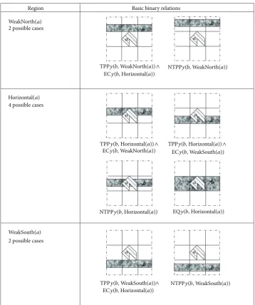
5.2. Basic Binary Relations of the Hybrid Model. In this section, we shall demonstrate how we come up with all possible binary direction relations for the hybrid model. All the possible basic binary relations for each horizontal set are

shown in Figure 7. The notations that will be used in this

section are as follows.

(i) RELy(b,Z)is any basic binary relation between𝑏and

the horizontally partitioned region,𝑍.

(ii) RELx(b,Z)is any basic binary relation between𝑏and

the vertically partitioned region,𝑍.

Based on Figure 7, the total number of possible binary

relations for the hybrid model in the y-direction is [(2 +

4 + 2) + (2 × 4) + (2 × 2) + (4 × 2) + (2 × 4 × 2)]which equals 44 cases. However, due to the single-piece condition, the following rules apply.

Rule 1. ¬(b⊆WeakNorth(a)∧ 𝑏 ⊆WeakSouth(a)).

Rule 2. Assume 𝑈 to be {WeakNorth(a), Horizontal(a),

𝑎 𝑎 𝑎

𝑎

𝑏

𝑎

𝑎

𝑎 𝑎

𝑏

𝑏 𝑏 𝑏

𝑏 𝑏

𝑏

DC(𝑎, 𝑏) EC(𝑎, 𝑏) PO(𝑎, 𝑏) EQ(_{𝑎, 𝑏})

𝑎disconnected from𝑏 _𝑎externally connected to𝑏 𝑎partial overlapping_{𝑏 𝑎}equals_𝑏

TTP(𝑎, 𝑏)

𝑎tangential proper

part of_𝑏

TTPi(𝑎, 𝑏)

𝑏tangential proper

part of𝑎

NTTP(𝑎, 𝑏)

𝑎nontangential proper

part of𝑏

NTTPi(_{𝑎, 𝑏})

𝑏nontangential proper

part of_𝑎

Figure 6: 8 basic JEPD RCC binary relations [13].

Table 1: Spatial relations defined in terms of C(𝑎, 𝑏)[18].

Relations Semantics Definition

DC(𝑎, 𝑏) ais disconnected fromb ¬C(𝑎, 𝑏)

P(𝑎, 𝑏) ais part ofb ∀_𝑒[C(𝑒, 𝑎) → C(𝑒, 𝑏)]

PP(𝑎, 𝑏) ais a proper part ofb P(𝑎, 𝑏) ∧ ¬P(𝑏, 𝑎)

EQ(𝑎, 𝑏) ais identical withb P(𝑎, 𝑏) ∧P(𝑏, 𝑎)

O(𝑎, 𝑏) aoverlapsb ∃_𝑒[P(𝑒, 𝑎) ∧P(𝑒, 𝑏)]

DR(𝑎, 𝑏) ais discrete fromb ¬O(𝑎, 𝑏)

PO(𝑎, 𝑏) apartially overlapsb O(𝑎, 𝑏) ∧ ¬P(𝑎, 𝑏) ∧ ¬P(𝑏, 𝑎)

EC(𝑎, 𝑏) ais externally connected tob C(𝑎, 𝑏) ∧ ¬O(𝑎, 𝑏)

TPP(𝑎, 𝑏) ais a tangential proper part ofb PP(𝑎, 𝑏) ∧ ∃_𝑒[EC(𝑒, 𝑎) ∧EC(𝑒, 𝑏)]

NTPP(𝑎, 𝑏) ais a nontangential proper part ofb PP(𝑎, 𝑏) ∧ ¬ ∃_𝑒[EC(𝑒, 𝑎) ∧EC(𝑒, 𝑏)]

If NTPP𝑦(𝑏, 𝑅)where𝑅 ∈ 𝑈then¬(NTPP𝑦(𝑏, 𝑅)∧

REL𝑦(𝑏, 𝑆)),

where𝑆 ∈ 𝑈 − 𝑅, or¬(NTPP𝑦(𝑏, 𝑅)∧REL𝑦(𝑏, 𝑆)∧

REL𝑦(𝑏, 𝑇)),

whereT∈ 𝑈 − 𝑆.

Rule 3. Assume𝑈to be{WeakNorth(a), WeakSouth(a)}.

If (TPP𝑦(𝑏,Horizontal(𝑎))∧EC𝑦(𝑏, 𝑅)), where𝑅 ∈ 𝑈,

then¬(TPP𝑦(𝑏,Horizontal)∧EC𝑦(𝑏, 𝑅)∧REL𝑦(𝑏, 𝑆)),

where𝑆 ∈ 𝑈 − 𝑅.

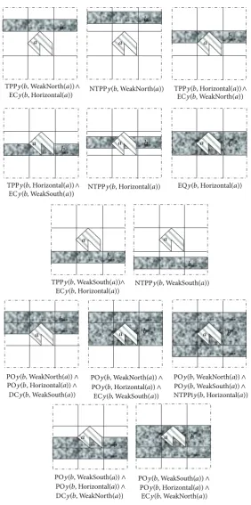
Based on the rules above, the total number of feasible

binary relations for single-piece regions in they-direction is

(44-4-23-4) which equals 13 cases. The thirteen feasible and jointly exhaustive binary relations for the hybrid model are

depicted inFigure 8. This means that, in the hybrid model, the

number of jointly exhaustive binary relations (in both the𝑥

-and𝑦-directions) that hold between two single-piece regions

will be13 × 13. This concurs with the13 × 13basic relations

in theRectangle Algebra Model[16,17].

6. Combined Mereological, Topological, and

Cardinal Direction Relations

Mereology (from the Greek𝜇𝜀𝜌o𝜍, “part”) is the theory of

parthood relations: of the relations of part to whole and the

relations, of part to part within a whole [36]. In this section,

we shall make two distinctions: “whole and part” cardinal directions, as well as “weak and expressive” relations. We shall

rewrite the notations used in our previous paper [29].𝑃R(b,a)

means that only part of the destination extended region,b,

is in tile R(a). The direction relation 𝐴R(b, a) means that

Region Basic binary relations

2 possible cases

4 possible cases

2 possible cases WeakNorth( )

Horizontal( )

WeakSouth( )

𝑎

𝑎

𝑎

𝑎

𝑎

𝑎

𝑎 𝑏

𝑏

𝑎

𝑎 𝑎

𝑎 𝑏

𝑏 _𝑏

𝑏 𝑏 𝑏

TPP𝑦(𝑏, WeakNorth(𝑎))∧ NTPP𝑦(𝑏, WeakNorth(𝑎))

EC𝑦(𝑏, Horizontal(𝑎))

TPP_𝑦(_𝑏, Horizontal(_𝑎))_∧ TPP_𝑦(_𝑏, Horizontal(_𝑎))_∧

EC𝑦(𝑏, WeakNorth(𝑎)) EC𝑦(𝑏, WeakSouth(𝑎))

NTPP𝑦(𝑏, Horizontal(𝑎)) EQ𝑦(𝑏, Horizontal(𝑎))

TPP𝑦(𝑏, WeakSouth(𝑎))∧

EC_𝑦(_𝑏, Horizontal(_𝑎))

NTPP_𝑦(_𝑏, WeakSouth(_𝑎))

Figure 7: Possible basic binary relations for each horizontally partitioned region (note: it will be similar for vertically partitioned region).

an example, when𝑏is completely in the South-East tile ofa,

this direction relation can be represented as shown below:

𝐴SE(𝑏, 𝑎) = ¬𝑃N(𝑏, 𝑎) ∧ ¬𝑃NE(𝑏, 𝑎) ∧ ¬𝑃NW(𝑏, 𝑎)

∧ ¬𝑃S(𝑏, 𝑎) ∧ 𝑃SE(𝑏, 𝑎) ∧ ¬𝑃SW(𝑏, 𝑎)

∧ ¬𝑃W(𝑏, 𝑎) ∧ ¬𝑃E(𝑏, 𝑎) ∧ ¬𝑃O(𝑏, 𝑎) .

(4)

The “whole and weak” direction relations are defined in terms of horizontal and vertical sets:

(i)𝐴N(𝑏, 𝑎) ≡WeakNorth(𝑏, 𝑎)∧Vertical(𝑏, 𝑎),

(ii)𝐴NE(𝑏, 𝑎) ≡WeakNorth(𝑏, 𝑎)∧WeakEast(𝑏, 𝑎),

(iii)𝐴NW(𝑏, 𝑎) ≡WeakNorth(𝑏, 𝑎)∧WeakWest(𝑏, 𝑎),

(iv)𝐴S(𝑏, 𝑎) ≡WeakSouth(𝑏, 𝑎)∧Vertical(𝑏, 𝑎),

(v)𝐴SE(𝑏, 𝑎) ≡WeakSouth(𝑏, 𝑎)∧WeakEast(𝑏, 𝑎),

(vi)𝐴SW(𝑏, 𝑎) ≡WeakSouth(𝑏, 𝑎)∧WeakWest(𝑏, 𝑎),

(vii)𝐴E(𝑏, 𝑎) ≡Horizontal(𝑏, 𝑎)∧WeakEast(𝑏, 𝑎),

(viii)𝐴W(𝑏, 𝑎) ≡Horizontal(𝑏, 𝑎)∧WeakWest(𝑏, 𝑎),

(ix)𝐴O(𝑏, 𝑎) ≡Horizontal(𝑏, 𝑎)∧Vertical(𝑏, 𝑎).

The “whole and expressive” direction relations are defined in terms of expressive horizontal and vertical sets. A general form of such direction relation can be represented as follows:

REL𝑦(𝑏,H(𝑎))[𝐴

𝑅(𝑏, 𝑎)]REL𝑥(𝑏,V(𝑎))

≡REL𝑦 (𝑏,H(𝑎)) ∧REL𝑥 (𝑏,V(𝑎)) ,

(5)

where H(a) and V(a) are horizontally and vertically

parti-tioned regions for𝑎, respectively, whereb⊆R(a) and R(a)

, WeakNorth(

TPP𝑦(𝑏, WeakNorth(𝑎

𝑎 𝑎 𝑎

𝑎 𝑎

𝑎

𝑎

𝑎 𝑎

𝑎 𝑎

𝑎

𝑎 ))∧

EC𝑦(𝑏, Horizontal(𝑎)) TPP𝑦(𝑏, Horizontal(𝑎))∧

TPP𝑦(𝑏, Horizontal(𝑎))∧

EC𝑦(𝑏, WeakNorth(𝑎))

EC𝑦(𝑏, WeakSouth(𝑎))

EC𝑦(𝑏, WeakSouth(𝑎))

NTPP_𝑦(_𝑏, Horizontal(_𝑎)) EQ𝑦(𝑏, Horizontal(𝑎))

TPP𝑦(𝑏, WeakSouth(𝑎))∧

EC𝑦(𝑏

𝑏 𝑏

𝑏

𝑏 𝑏

𝑏

𝑏

𝑏

𝑏

𝑏 𝑏

𝑏 𝑏

, Horizontal(𝑎

𝑎

𝑎 _𝑎𝑎 𝑎𝑎

))

NTPP𝑦(𝑏 𝑎))

NTPP𝑦(𝑏, WeakSouth(𝑎))

PO𝑦(𝑏, WeakNorth( ))∧

PO𝑦(𝑏, Horizontal( ))∧

DC𝑦(𝑏, WeakSouth(𝑎))

PO𝑦(𝑏, WeakNorth( ))∧

PO𝑦(𝑏, Horizontal( ))∧

PO𝑦(𝑏, WeakNorth( ))∧

PO𝑦(𝑏, WeakSouth( ))∧

NTPPi𝑦(𝑏, Horizontal(𝑎))

PO𝑦(𝑏, WeakSouth( ))∧

PO_𝑦(_𝑏, Horizontal( ))_∧

DC𝑦(𝑏, WeakNorth(𝑎

𝑎 PO𝑦(𝑏, Horizontal( ))𝑎 ∧

𝑎 𝑎

))

PO_𝑦(_𝑏, WeakSouth( ))_∧

EC_𝑦(_𝑏, WeakNorth(_𝑎))

Figure 8: Thirteen feasible and jointly exhaustive binary relations in they-direction for the hybrid model (note: this will be similar for

7. Composition Table

Composition is a common inference mechanism for a wide range of relations and has been exploited for automated reasoning. It has been employed for reasoning about temporal

descriptions of events based on intervals [37],

topologi-cal relations [5, 38–42], direction relations [1,24,29,30],

and combined topological relations with cardinal direction

relations [19]. To reiterate, one of the main advantages of

using composition tables is that they can lead to tractable

computation of significant classes of inference [25].

Given the relation between 𝑎 and b and the relation

between𝑏andc, a composition table allows for concluding

the relation between𝑎and𝑐. Bennett [41] defines the concept

of the composition of two binary relations as follows.

Given a theory Θ which is used to define a set 𝛽

of mutually exhaustive and pairwise disjoint dyadic

relations (i.e., a basis set), the composition, Comp(𝑅₁,

𝑅₂), of two relations𝑅₁and𝑅₂which are taken from

ß is defined to be the disjunction of all relations𝑅₃

in ß, such that, for arbitrary constants𝑎,𝑏, and𝑐, the

formula𝑅₁(𝑎, 𝑏)∧𝑅₂(𝑏, 𝑐)∧𝑅₃(𝑎, 𝑐)is consistent with

Θ.

7.1. Composition of Regions with Parts. In our previous paper

[29], the method for computing the composition of cardinal

direction relations for part regions is not robust enough, because it does not hold for all cases. In order to address this problem, we introduce a formula (obtained through case analyses) for computing the composition of cardinal direction relations. The basis of the formula is to consider

the direction relation between𝑎and each individual part of

𝑏followed by the direction relation between each individual

part of𝑏andc.

Assume that the region covers one or moretilesof region

𝑎while region𝑐covers one or moretilesof𝑏.The direction

relation between𝑎and𝑏is𝑅(𝑏, 𝑎)while the direction relation

between 𝑏 and c is 𝑆(𝑐, 𝑏). The composition of direction

relations could be written as follows:

𝑅(𝑏, 𝑎) ∧ 𝑆(𝑐, 𝑏) . (6)

Firstly, establish the direction relation between𝑎and each

individual part ofb:

𝑅(𝑏, 𝑎) ∧ 𝑆(𝑐, 𝑏)

≡ [𝑅₁(𝑏₁, 𝑎) ∧ 𝑅₂(𝑏₂, 𝑎) ⋅ ⋅ ⋅ ∧ 𝑅_𝑘(𝑏_𝑘, 𝑎)] ∧ [𝑆 (𝑐, 𝑏)] ,

(7)

where1 ≤ 𝑘 ≤ 9.

Consider the direction relation of each individual part of

𝑏and𝑐. Equation (7) becomes

[[𝑅₁(𝑏₁, 𝑎) ∧ 𝑆₁₁(𝑐₁, 𝑏₁)] ∨ [𝑅₁(𝑏₁, 𝑎) ∧ 𝑆₁₂(𝑐₂, 𝑏₁)] ⋅ ⋅ ⋅ ∨ [𝑅₁(𝑏₁, 𝑎) ∧ 𝑆_1𝑚(𝑐_1𝑚, 𝑏₁)]]

∧ [[𝑅2(𝑏2, 𝑎) ∧ 𝑆21(𝑐1, 𝑏2)] ∨ [𝑅2(𝑏2, 𝑎) ∧ 𝑆22(𝑐2, 𝑏2)] ⋅ ⋅ ⋅

∨ [𝑅₂(𝑏₂, 𝑎) ∧ 𝑆_2𝑚(𝑐_2𝑚, 𝑏₂)]]

∧ ⋅ ⋅ ⋅ [[𝑅_𝑘(𝑏_𝑘, 𝑎) ∧ 𝑆_𝑘1(𝑐₁, 𝑏_𝑘)] ∨ [𝑅_𝑘(𝑏_𝑘, 𝑎) ∧ 𝑆_𝑘2(𝑐₂, 𝑏_𝑘)] ⋅ ⋅ ⋅ ∨ [𝑅𝑘(𝑏𝑘, 𝑎) ∧ 𝑆𝑘𝑚(𝑐𝑘𝑚, 𝑏𝑘)]] ,

(8)

where1 ≤ 𝑘, 𝑚 ≤ 9.

7.2. Composition of Weak Direction Relations. Firstly, we shall demonstrate how to apply the formula for the composition of weak direction relations followed by more expressive direction relations.

Type 1. 𝐴_𝑅(𝑏, 𝑎) ∧ 𝐴_𝑅(𝑐, 𝑏).

Find the composition of𝐴O(𝑏, 𝑎) ∧ 𝐴SW(𝑐, 𝑏).

Use (8) with𝑘 = 1and𝑚 = 1:

𝑅₁(𝑏₁, 𝑎) ∧ 𝑆₁₁(𝑐₁, 𝑏₁) ≡ 𝐴O(𝑏, 𝑎) ∧ 𝐴SW(𝑐, 𝑏)

≡ [Horizontal(𝑏, 𝑎) ∧Vertical(𝑏, 𝑎)]

∧ [WeakSouth(𝑐, 𝑏) ∧WeakWest(𝑐, 𝑏)]

≡ [Horizontal(𝑏, 𝑎) ∧WeakSouth(𝑐, 𝑏)]

∧ [Vertical(𝑏, 𝑎) ∧WeakWest(𝑐, 𝑏)] .

(9)

The outcome of the composition is

[Horizontal(𝑐, 𝑎) ∨WeakSouth(𝑐, 𝑎)]

∧ [Vertical(𝑐, 𝑎) ∨WeakWest(𝑐, 𝑎)] . (10)

This means that the region c⊆O(a) ∨W(a) ∨S(a)∨

SW(a).

Type 2. 𝐴_𝑅(𝑏, 𝑎) ∧ 𝑃_𝑅(𝑐, 𝑏).

Find the composition of𝐴E(𝑏, 𝑎) ∧ [𝑃NW(𝑐, 𝑏) ∧ 𝑃N(𝑐, 𝑏)].

Use (8) withk= 1, and1 ≤ 𝑚 ≤ 2:

[[𝑅₁(𝑏₁, 𝑎) ∧ 𝑆₁₁(𝑐₁, 𝑏₁)] ∨ [𝑅₁(𝑏₁, 𝑎) ∧ 𝑆₁₂(𝑐₂, 𝑏₁)]] ≡ [[𝐴_𝐸(𝑏, 𝑎) ∧ 𝐴_𝑁𝑊(𝑐₁, 𝑏)] ∨ [𝐴_𝐸(𝑏, 𝑎) ∧ 𝐴_𝑁(𝑐₂, 𝑏)]]

≡ [[Horizontal(𝑏, 𝑎) ∧WeakEast(𝑏, 𝑎)]

∧ [WeakNorth(𝑐₁, 𝑏) ∧WeakWest(𝑐₁, 𝑏)]]

2 2

≡ [[Horizontal(𝑏, 𝑎) ∧WeakNorth(𝑐₁, 𝑏)]

∧ [WeakEast(𝑏, 𝑎) ∧WeakWest(𝑐₁, 𝑏)]]

∨ [[Horizontal(𝑏, 𝑎) ∧WeakNorth(𝑐₂, 𝑏)]

∧ [WeakEast(𝑏, 𝑎) ∧Vertical(𝑐₂, 𝑏)]] .

(11)

The outcome of the composition is

[[Horizontal(𝑐₁, 𝑎) ∨WeakNorth(𝑐₁, 𝑎)]

∧ [WeakEast(𝑐₁, 𝑎) ∨Vertical(𝑐₁, 𝑎) ∨WeakWest(𝑐₁, 𝑎)]]

∨ [[Horizontal(𝑐₂, 𝑎) ∨WeakNorth(𝑐₂, 𝑎)]

∧ [WeakEast(𝑐₂, 𝑎)]] .

(12)

Viewing the fact that𝑐₁⊂ 𝑐and𝑐₂⊂ 𝑐, the above outcome

can be written as

[[Horizontal(𝑐, 𝑎) ∨WeakNorth(𝑐, 𝑎)]

∧ [WeakEast(𝑐, 𝑎) ∨Vertical(𝑐, 𝑎) ∨WeakWest(𝑐, 𝑎)]] .

(13)

This means that the region 𝑐 ⊆E(a)∨O(a)∨W(a)∨

NE(a)∨N(a)∨NW(a).

Type 3. 𝑃_𝑅(𝑏, 𝑎)∧ 𝐴_𝑅(𝑐, 𝑏).

Find the composition of[𝑃O(𝑏1, 𝑎)∧𝑃N(𝑏2, 𝑎)]∧𝐴NE(𝑐, 𝑏).

Establish the relationship between𝑐and each individual part

of𝑏. In this case,𝐴NE(𝑐, 𝑏),𝑃NE(𝑐, 𝑏1) and𝑃NE(𝑐, 𝑏2) holds

(this is not necessarily true for all cases).

Use (8) with1 ≤ 𝑘 ≤ 2and𝑚 = 1.

[[𝑃𝑅1(𝑏1, 𝑎)] ∧ [𝑃𝑅11(𝑐1, 𝑏1)]] ∧ [[𝑃_𝑅2(𝑏₂, 𝑎)] ∧ [𝑃_𝑅21(𝑐₁, 𝑏₂)]] ≡ [[𝑃O(𝑏1, 𝑎)] ∧ [𝑃NE(𝑐, 𝑏)]]

∧ [[𝑃N(𝑏2, 𝑎)] ∧ [𝑃NE(𝑐, 𝑏)]] .

(14)

Therefore, the above composition can be rewritten as

[[𝑃O(𝑏1, 𝑎)] ∧ [𝑃NE(𝑐, 𝑏1)]] ∧ [[𝑃N(𝑏2, 𝑎)] ∧ [𝑃NE(𝑐, 𝑏2)]]

≡ [[Horizontal(𝑏₁, 𝑎) ∧Vertical(𝑏₁, 𝑎)]

Boundaries of minimal bounding box for region𝑎 𝑎

Boundaries of minimal bounding box for region

𝑏2

𝑏

𝑏 1

𝑐

Figure 9: An example.

∧ [WeakNorth(𝑐, 𝑏₁) ∧WeakEast(𝑐, 𝑏₁)]]

∧ [[WeakNorth(𝑏₂, 𝑎) ∧Vertical(𝑏₂, 𝑎)]

∧ [WeakNorth(𝑐, 𝑏₂) ∧WeakEast(𝑐, 𝑏₂)]]

≡ [[Horizontal(𝑏₁, 𝑎) ∧WeakNorth(𝑐, 𝑏₁)]

∧ [Vertical(𝑏₁, 𝑎) ∧WeakEast(𝑐, 𝑏₁)]]

∧ [[WeakNorth(𝑏₂, 𝑎) ∧WeakNorth(𝑐, 𝑏₂)]

∧ [Vertical(𝑏₂, 𝑎) ∧WeakEast(𝑐, 𝑏₂)]] .

(15)

The outcome of the composition is

[[Horizontal(𝑐, 𝑎) ∨WeakNorth(𝑐, 𝑎)]

∧ [WeakEast(𝑐, 𝑎) ∨Vertical(𝑐, 𝑎)]]

∧ [[NTPP_𝑦(𝑐,WeakNorth(𝑎))]

∧ [WeakEast(𝑐, 𝑎) ∨Vertical(𝑐, 𝑎)]]

= [[NTPP_𝑦(𝑐,WeakNorth(𝑎))]

∧ [WeakEast(𝑐, 𝑎) ∨Vertical(𝑐, 𝑎)]] .

(16)

This means that the𝑌_min(𝑐)of the minimal bounding box

for region𝑐is greater than𝑌_max(𝑎)of the minimal bounding

box for region𝑎and𝑐 ⊆NE(𝑎) ∨N(𝑎).

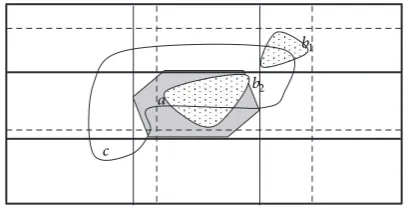
Type 4. 𝑃_𝑅(𝑏, 𝑎) ∧ 𝑃_𝑅(𝑐, 𝑏). Find the composition of

[𝑃O(𝑏1, 𝑎) ∧ 𝑃NE(𝑏2, 𝑎)] ∧ [𝑃O(𝑐, 𝑏) ∧ 𝑃W(𝑐, 𝑏) ∧ 𝑃SW(𝑐, 𝑏)] .

(17)

Figure 9has been drawn for this example. Establish the

Use (8) with1 ≤ 𝑘 ≤ 2; the value of𝑚₁for𝑏₁is1 ≤ 𝑚₁≤

4, while the value𝑚₂for𝑏₂is1 ≤ 𝑚₂≤ 7:

[[𝑃𝑅1(𝑏1, 𝑎) ∧ 𝑃𝑅11(𝑐1, 𝑏1)] ∨ [𝑃𝑅1(𝑏1, 𝑎) ∧ 𝑃𝑅12(𝑐2, 𝑏1)] ∨ [𝑃_𝑅1(𝑏₁, 𝑎) ∧ 𝑃_𝑅13(𝑐₃, 𝑏₁)]

∨ [𝑃_𝑅1(𝑏₁, 𝑎) ∧ 𝑃_𝑅14(𝑐₄, 𝑏₁)]]

∧ [[𝑃_𝑅2(𝑏₂, 𝑎) ∧ 𝑃_𝑅21(𝑐₁, 𝑏₂)] ∨ [𝑃_𝑅2(𝑏₂, 𝑎) ∧ 𝑃_𝑅22(𝑐₂, 𝑏₂)] ∨ [𝑃_𝑅2(𝑏₂, 𝑎) ∧ 𝑃_𝑅25(𝑐₅, 𝑏₂)] ∨ [𝑃_𝑅2(𝑏₂, 𝑎) ∧ 𝑃_𝑅26(𝑐₆, 𝑏₂)] ∨ [𝑃_𝑅2(𝑏₂, 𝑎) ∧ 𝑃_𝑅27(𝑐₇, 𝑏₂)]]

≡ [[𝑃O(𝑏1, 𝑎) ∧ 𝑃S(𝑐1, 𝑏1)] ∨ [𝑃O(𝑏1, 𝑎) ∧ 𝑃SW(𝑐2, 𝑏1)]

∨ [𝑃O(𝑏1, 𝑎) ∧ 𝑃W(𝑐3, 𝑏1)] ∨ [𝑃O(𝑏1, 𝑎) ∧ 𝑃O(𝑐4, 𝑏1)]]

∧ [[𝑃NE(𝑏2, 𝑎) ∧ 𝑃NE(𝑐1, 𝑏2)] ∨ [𝑃NE(𝑏2, 𝑎) ∧ 𝑃N(𝑐2, 𝑏2)] ∨ [𝑃NE(𝑏2, 𝑎) ∧ 𝑃NW(𝑐3, 𝑏2)]

∨ [𝑃NE(𝑏2, 𝑎) ∧ 𝑃E(𝑐4, 𝑏2)] ∨ [𝑃NE(𝑏2, 𝑎) ∧ 𝑃O(𝑐5, 𝑏2)] ∨ [𝑃NE(𝑏2, 𝑎) ∧ 𝑃W(𝑐6, 𝑏2)]

∨ [𝑃NE(𝑏2, 𝑎) ∧ 𝑃SW(𝑐7, 𝑏2)]] .

(18)

In part (1) of the above composition, 𝑐₁,𝑐₂,𝑐₃,𝑐₄ ⊂ 𝑐.

To simplify the composition, we consider the combined

horizontal and vertical sets of all the parts of𝑐.Thus, we have

the following:

[WeakNorth(𝑏₁, 𝑎) ∧WeakEast(𝑏₁, 𝑎)]

∧ [[Horizontal(𝑐, 𝑏₁) ∨WeakSouth(𝑐, 𝑏₁)]

∧ [Vertical(𝑐, 𝑏₁) ∨WeakWest(𝑐, 𝑏₁)]]

≡ [[WeakNorth(𝑏₁, 𝑎)]

∧ [Horizontal(𝑐, 𝑏₁) ∨WeakSouth(𝑐, 𝑏₁)]]

∧ [[WeakEast(𝑏₁, 𝑎)]

∧ [Vertical(𝑐, 𝑏₁) ∨WeakWest(𝑐, 𝑏₁)]]

= [WeakNorth(𝑐, 𝑎) ∨Horizontal(𝑐, 𝑎)

∨WeakSouth(𝑐, 𝑎)]

∧ [WeakEast(𝑐, 𝑎) ∨Vertical(𝑐, 𝑎) ∨WeakWest(𝑐, 𝑎)] .

(19)

In part(2)of the above composition,𝑐₁,𝑐₂,𝑐₃,𝑐₄,𝑐₅,𝑐₆,

𝑐₇⊂ 𝑐. The simplified version of the composition is as follows:

[Horizontal(𝑏₂, 𝑎) ∧Vertical(𝑏₂, 𝑎)]

∧ [[WeakNorth(𝑐, 𝑏₂) ∨Horizontal(𝑐, 𝑏₂)

∨WeakSouth(𝑐, 𝑏₂)]

∧ [WeakEast(𝑐, 𝑏₂) ∨Vertical(𝑐, 𝑏₂)

∨WeakWest(𝑐, 𝑏₂)]]

≡ [[Horizontal(𝑏₂, 𝑎)]

∧ [WeakNorth(𝑐, 𝑏₂) ∨Horizontal(𝑐, 𝑏₂)

∨WeakSouth(𝑐, 𝑏₂)]]

∧ [[Vertical(𝑏₂, 𝑎)]

∧ [WeakEast(𝑐, 𝑏₂) ∨Vertical(𝑐, 𝑏₂)

∨WeakWest(𝑐, 𝑏₂)]]

= [[WeakNorth(𝑐, 𝑎) ∨Horizontal(𝑐, 𝑎)

∨WeakSouth(𝑐, 𝑎)]]

∧ [WeakEast(𝑐, 𝑎) ∨Vertical(𝑐, 𝑎)

∨WeakWest(𝑐, 𝑎)]] .

(20)

The final outcome of the composition is part(1) ∧part

(2)is equivalent to

[WeakNorth(𝑐, 𝑎) ∨Horizontal(𝑐, 𝑎) ∨WeakSouth(𝑐, 𝑎)]

∧ [WeakEast(𝑐, 𝑎) ∨Vertical(𝑐, 𝑎) ∨WeakWest(𝑐, 𝑎)] .

(21)

This means that the regionc⊆Uwhich is the union of all

the 9tilesof regiona. However, based onFigure 9, regionc ̸⊂

SW(a).

7.3. Composition of Expressive Direction Relations. We shall

use the following notations to represent the 13 binary

y-direction relations:

(i) REL1𝑦(𝑏, 𝑎)-NTPP𝑦(𝑏,WeakNorth(𝑎)),

(ii) REL2𝑦(𝑏, 𝑎)-TPP𝑦(𝑏,WeakNorth(𝑎))

∧EC𝑦(𝑏,Horizontal(𝑎)),

(iii) REL3𝑦(𝑏, 𝑎)-TPP𝑦(𝑏,Horizontal(𝑎))

∧EC𝑦(𝑏,WeakNorth(𝑎)),

(iv) REL4𝑦(𝑏, 𝑎)-TPP𝑦(𝑏,Horizontal(𝑎))

∧EC𝑦(𝑏,WeakSouth(𝑎)),

(v) REL5𝑦(𝑏, 𝑎)-NTPP𝑦(𝑏,Horizontal(𝑎)),

(vi) REL6𝑦(𝑏, 𝑎)-EQy(𝑏,Horizontal(𝑎)),

(vii) REL7𝑦(𝑏, 𝑎)-NTPP𝑦(𝑏,WeakSouth(𝑎)),

(viii) REL8𝑦(𝑏, 𝑎)-TPP𝑦(𝑏,WeakSouth(𝑎))

∧PO𝑦(𝑏,Horizontal(𝑎))∧

DC𝑦(𝑏,WeakSouth(𝑎)),

(x) REL10𝑦(𝑏, 𝑎)-PO𝑦(𝑏,WeakNorth(𝑎))

∧PO𝑦(𝑏,Horizontal(𝑎))∧

EC𝑦(𝑏,WeakSouth(𝑎)),

(xi) REL11𝑦(𝑏, 𝑎)-PO𝑦(𝑏,WeakNorth(𝑎))

∧PO𝑦(𝑏,WeakSouth(𝑎))∧

NTPPi𝑦(𝑏,Horizontal(𝑎)),

(xii) REL12𝑦(𝑏, 𝑎)-PO𝑦(𝑏,WeakSouth(𝑎))

∧PO𝑦(𝑏,Horizontal(𝑎))∧

DC𝑦(𝑏,WeakNorth(𝑎)),

(xiii) REL13𝑦(𝑏, 𝑎)-PO𝑦(𝑏,WeakSouth(𝑎))

∧PO𝑦(𝑏,Horizontal(𝑎))∧

EC𝑦(𝑏,WeakNorth(𝑎)).

Similar notations will be used to represent the 13 binary x-direction relations (WeakNorth is replaced by WeakEast, HorizontalwithVertical,andWeakSouthbyWeakWest).

Example 1. Find the composition of the following:

[[REL3𝑦(𝑏₁,𝑎)_[𝑃

O(𝑏1, 𝑎)]REL3𝑥(𝑏1,𝑎)]

∧ [REL2𝑦(𝑏2,𝑎)_[𝑃

NE(𝑏2, 𝑎)]REL2𝑥(𝑏2,𝑎)]]

∧ [REL1𝑦(𝑐,𝑏)_[𝐴

N(𝑐, 𝑏)]REL5𝑥(𝑐,𝑏)] .

(22)

Establish the direction relation between 𝑐 and each

individual part of𝑏. Use (8), with1 ≤ 𝑘 ≤ 2and1 ≤ 𝑚₁≤ 2,

and1 ≤ 𝑚₂≤ 2:

[[𝑃_𝑅1(𝑏₁, 𝑎)] ∧ [𝑃_𝑅11(𝑐₁, 𝑏₁) ∨ 𝑃_𝑅12(𝑐₂, 𝑏₁)]]

∧ [[𝑃_𝑅2(𝑏₂, 𝑎)] ∧ [𝑃_𝑅21(𝑐₁, 𝑏₂) ∨ 𝑃_𝑅22(𝑐₂, 𝑏₂)]] . (23)

Use (5), and the above composition can be rewritten in

the following expressive form:

[[REL3𝑦 (𝑏₁, 𝑎) ∧REL3𝑥 (𝑏₁, 𝑎)]]

∧ [[REL1𝑦 (𝑐₁, 𝑏₁) ∧REL3𝑥 (𝑐₁, 𝑏₁)]

∨ [REL1𝑦 (𝑐₂, 𝑏₁) ∧REL2𝑥 (𝑐₂, 𝑏₁)]]

∧ [[REL2𝑦 (𝑏₂, 𝑎) ∧REL2𝑥 (𝑏₂, 𝑎)]]

∧ [[REL1𝑦 (𝑐₁, 𝑏₂) ∧REL8𝑥 (𝑐₁, 𝑏₂)]

∨ [REL1𝑦 (𝑐₂, 𝑏₂) ∧REL4𝑥 (𝑐₂, 𝑏₂)]]

≡ [REL3𝑦 (𝑏₁, 𝑎) ∧ [REL1𝑦 (𝑐₁, 𝑏₁) ∨REL1𝑦 (𝑐₂, 𝑏₁)]]

∧ [REL3𝑥 (𝑏₁, 𝑎) ∧ [REL3𝑥 (𝑐₁, 𝑏₁) ∨REL2𝑥 (𝑐₂, 𝑏₁)]]

∧ [REL2𝑦 (𝑏₂, 𝑎) ∧ [REL1𝑦 (𝑐₁, 𝑏₂) ∨REL1𝑦 (𝑐₂, 𝑏₂)]]

∧ [REL2𝑥 (𝑏₂, 𝑎) ∧ [REL8𝑥 (𝑐₁, 𝑏₂) ∨REL4𝑥 (𝑐₂, 𝑏₂)]] . (24)

1 2

outcome of the composition can be written as follows:

REL1𝑦 (𝑐, 𝑎) ∧ [REL2𝑥 (𝑐, 𝑎) ∨REL3𝑥 (𝑐, 𝑎)] ∧REL1𝑦 (𝑐, 𝑎)

∧ [REL2𝑥 (𝑐, 𝑎) ∨REL3𝑥 (𝑐, 𝑎)

∨REL6𝑥 (𝑐, 𝑎) ∨REL13𝑥 (𝑐, 𝑎)]

=REL1𝑦 (𝑐, 𝑎) ∧ [REL2𝑥 (𝑐, 𝑎) ∨REL3𝑥 (𝑐, 𝑎)] . (25)

The outcome of the composition is:

NTPP𝑦 (𝑐,WeakNorth(𝑎))

∧ [TPP𝑥 (𝑐,WeakEast(𝑎)) ∧EC𝑦 (𝑐,Horizontal(𝑎))

∨TPP𝑥 (𝑐,Vertical(𝑎)) ∧EC𝑦 (𝑐,Horizontal(𝑎))] . (26)

Example 2. This example is similar to the fourth example in the previous section of this paper.

Find the composition of

[𝑃O(𝑏1, 𝑎) ∧ 𝑃NE(𝑏2, 𝑎)]

∧ [𝑃O(𝑐, 𝑏) ∧ 𝑃W(𝑐, 𝑏) ∧ 𝑃SW(𝑐, 𝑏)] .

(27)

Establish the direction relation between 𝑐 and each

individual part of𝑏.Use (8), with 1≤k≤2 and 1≤ 𝑚₁ ≤

4, and 1≤ 𝑚₂≤7.

The composition in expressive form will be as follows.

For part𝑏₁,

[[REL2𝑦 (𝑏₁, 𝑎) ∧REL2𝑥 (𝑏₁, 𝑎)]]

∧ [[REL4𝑦 (𝑐₁, 𝑏₁) ∧REL4𝑥 (𝑐₁, 𝑏₁)]

∨ [REL8𝑦 (𝑐₂, 𝑏₁) ∧REL4𝑥 (𝑐₂, 𝑏₁)]

∨ [REL4𝑦 (𝑐₃, 𝑏₁) ∧REL8𝑥 (𝑐₃, 𝑏₁)]

∨ [REL8𝑦 (𝑐₄, 𝑏₁) ∧REL8𝑥 (𝑐₄, 𝑏₁)]] .

(28)

The regions𝑐₁,𝑐₂,𝑐₃,𝑐₄⊂ 𝑐; the above composition can be

written as follows:

[REL2𝑦 (𝑏₁, 𝑎)

∧ [REL4𝑦 (𝑐, 𝑏₁) ∨REL8𝑦 (𝑐, 𝑏₁)

∨REL4𝑦 (𝑐, 𝑏1) ∨REL8𝑦 (𝑐, 𝑏1)]]

∧ [REL2𝑥 (𝑏₁, 𝑎)

∧ [REL4𝑥 (𝑐, 𝑏₁) ∨REL4𝑥 (𝑐, 𝑏₁)

∨REL8𝑥 (𝑐, 𝑏₁) ∨REL8𝑥 (𝑐, 𝑏₁)]]

= [REL2𝑦 (𝑐, 𝑎) ∨REL3𝑦 (𝑐, 𝑎)

∨REL6𝑦 (𝑐, 𝑎) ∨REL13𝑦 (𝑐, 𝑎)]

∧ [REL2𝑥 (𝑐, 𝑎) ∨REL3𝑥 (𝑐, 𝑎)

∨REL6𝑥 (𝑐, 𝑎) ∨REL13𝑥 (𝑐, 𝑎)] .

For part𝑏₂

[[REL3𝑦 (𝑏₂, 𝑎) ∧REL3𝑥 (𝑏₂, 𝑎)]]

∧ [[REL8𝑦 (𝑐₁, 𝑏₂) ∧REL7𝑥 (𝑐₁, 𝑏₂)]

∨ [REL6𝑦 (𝑐₂, 𝑏₂) ∧REL8𝑥 (𝑐₂, 𝑏₂)]

∨ [REL2𝑦 (𝑐₃, 𝑏₂) ∧REL8𝑥 (𝑐₃, 𝑏₂)]

∨ [REL2𝑦 (𝑐₄, 𝑏₂) ∧REL6𝑥 (𝑐₄, 𝑏₂)]

∨ [REL3𝑦 (𝑐₅, 𝑏₂) ∧REL6𝑥 (𝑐₅, 𝑏₂)]

∨ [REL3𝑦 (𝑐₆, 𝑏₂) ∧REL2𝑥 (𝑐₆, 𝑏₂)]

∨ [REL2𝑦 (𝑐₇, 𝑏₂) ∧REL2𝑥 (𝑐₇, 𝑏₂)]]

= [[REL2𝑦 (𝑐, 𝑎) ∨REL3𝑦 (𝑐, 𝑎)

∨REL5𝑦 (𝑐, 𝑎) ∨REL12𝑦 (𝑐, 𝑎)]

∧ [REL2𝑥 (𝑐, 𝑎) ∨REL3𝑥 (𝑐, 𝑎)

∨REL4𝑥 (𝑐, 𝑎) ∨REL5𝑥 (𝑐, 𝑎)

∨REL7𝑥 (𝑐, 𝑎) ∨REL8𝑥 (𝑐, 𝑎) ∨REL12𝑥 (𝑐, 𝑎)]] . (29b)

The final outcome of the composition is the composition of

part𝑏₁(29a)∧part𝑏₂(29b).

ApplyRule 3from the earlier part of the paper, and we

will get the following:

[[REL2𝑦 (𝑐, 𝑎) ∨REL3𝑦 (𝑐, 𝑎)

∨REL6𝑦 (𝑐, 𝑎) ∨REL13𝑦 (𝑐, 𝑎)]

∧ [REL2𝑦 (𝑐, 𝑎) ∨REL3𝑦 (𝑐, 𝑎) ∨REL12𝑦 (𝑐, 𝑎)]

∧ [REL2𝑥 (𝑐, 𝑎) ∨REL3𝑥 (𝑐, 𝑎)

∨REL4𝑥 (𝑐, 𝑎) ∨REL8𝑥 (𝑐, 𝑎) ∨REL12𝑥 (𝑐, 𝑎)]

∧ [REL2𝑥 (𝑐, 𝑎) ∨REL3𝑥 (𝑐, 𝑎)

∨REL6𝑥 (𝑐, 𝑎) ∨REL13𝑥 (𝑐, 𝑎)]] .

(30)

We collapse some of the disjunction of relations:

REL6𝑦 (𝑐, 𝑎) ∨REL13𝑦 (𝑐, 𝑎) =REL13𝑦 (𝑐, 𝑎)

REL4𝑥 (𝑐, 𝑎) ∨REL8𝑥 (𝑐, 𝑎) ∨REL12𝑥 (𝑐, 𝑎) =REL12𝑦 (𝑐, 𝑎)

REL6𝑥 (𝑐, 𝑎) ∨REL13𝑥 (𝑐, 𝑎) =REL13𝑥 (𝑐, 𝑎) . (31)

Equation (30) becomes

[REL2𝑦 (𝑐, 𝑎) ∨REL3𝑦 (𝑐, 𝑎) ∨REL13𝑦 (𝑐, 𝑎)]

∧ [REL2𝑦 (𝑐, 𝑎) ∨REL3𝑦 (𝑐, 𝑎) ∨REL12𝑦 (𝑐, 𝑎)]

∧ [REL2𝑥 (𝑐, 𝑎) ∨REL3𝑥 (𝑐, 𝑎) ∨REL12𝑥 (𝑐, 𝑎)]

∧ [REL2𝑥 (𝑐, 𝑎) ∨REL3𝑥 (𝑐, 𝑎) ∨REL13𝑥 (𝑐, 𝑎)] . (32)

Region𝑐is single piece. Therefore, (32) becomes

[PO𝑦 (𝑐,WeakNorth(𝑎)) ∧PO𝑦 (𝑐,WeakSouth(𝑎))

∧NTPP𝑖𝑦 (𝑐,Horizontal(𝑎))] (33)

∧ [PO𝑥 (𝑐,WeakEast(𝑎)) ∧PO𝑥 (𝑐,WeakWest(𝑎))

∧NTPP𝑖𝑥 (𝑐,Vertical(𝑎))] . (34)

This means that the regionc⊆Uwhich is the union of all the

9tilesof region𝑎. As mentioned earlier, based onFigure 9,

regionc ̸⊂SW(a). Thus, the outcome of the composition for

weak relations (in the previous section) yields the same result as this composition. However, the computation for the latter is more tedious and complex when involving regions with many parts.

8. Existential Inference

The composition table inTable 2 is the result of transitive

inferences made about regions 𝑎 and c, given the hybrid

cardinal direction relations for regions 𝑎 and 𝑏 as well as

regions𝑏and𝑐. In the context of this paper, an existential

inference is the inference made about the spatial relation

between𝑎andb, given the relations between𝑐and𝑎or/and

the given relations between𝑐 and𝑏. We shall demonstrate

how our expressive hybrid cardinal direction model could be used to make several existential inferences which are not possible in existing models.

Example 3(Find𝑅(𝑏, 𝑎)such that𝑐 ⊂WeakNorth(𝑏) and𝑐 ⊂

WeakNorth(𝑎)). To answer this query, we must first specify

the expressive relation between𝑎andc.

There are two possible relations: TPP𝑦(c,WeakNorth(a))

or WeakNorth(c,a).If it is the former then composition is WeakNorth(b,a) ∧ WeakNorth(c,b) which means R(b,a) is WeakNorth(b,a).If it is the latter, there are several combina-tions:

(i) WeakNorth(𝑏, 𝑎)∧Horizontal(𝑐, 𝑏)

(ii) WeakNorth(𝑏, 𝑎)∧WeakSouth(𝑐, 𝑏)

(iii) Horizontal(𝑏, 𝑎)∧WeakNorth(𝑐, 𝑏)

(iv) WeakSouth(𝑏, 𝑎)∧WeakNorth(𝑐, 𝑏).

This means 𝑅(𝑏, 𝑎) are Horizontal(b,a) or WeakSouth

(b,a) when𝑐 ⊂WeakNorth(b) and𝑐 ⊂WeakNorth(a).

Example 4 (Find R(b,a) and S(c,b) such that T(a,c) is

¬[TPP𝑦(c,Horizontal(a)) ∧EC𝑦(c,WeakSouth(a))]). Based

onTable 2, 9 different compositions will yield the following outcome:

TPP𝑦(c,Horizontal(a))∧EC𝑦(c,WeakSouth(a))

The set of possible compositions,Q,is:

{REL1𝑦(𝑏, 𝑎)∧REL7𝑦(𝑐, 𝑏), REL2𝑦(𝑏, 𝑎)∧REL7𝑦(𝑐, 𝑏),

REL3𝑦(𝑏, 𝑎)∧REL7𝑦(𝑐, 𝑏), REL3𝑦(𝑏, 𝑎)∧REL8𝑦(𝑐, 𝑏),

REL5𝑦(𝑏, 𝑎)∧REL7𝑦(𝑐, 𝑏), REL5𝑦(𝑏, 𝑎)∧REL8𝑦(𝑐, 𝑏),

REL6𝑦(𝑏, 𝑎)∧REL4𝑦(𝑐, 𝑏), REL7𝑦(𝑏, 𝑎)∧REL1𝑦(𝑐, 𝑏),

set of all possible ordered pairs of𝑅and𝑆which satisfy the

above query will be𝑈 − 𝑄.

Example 5 (Find R(b,a) and S(c,b) such that T(a,c) is

PO𝑦(c,WeakSouth(a)) ∧ PO𝑦(c,Horizontal(a)) ∧ EC𝑦(c,

WeakNorth(a))). Based onTable 2, we have 4 pairs of𝑅and

𝑆 which satisfy 𝑇. They are: REL1y(b,a) ∧ REL7y(c,b),

REL2y(b,a) ∧ REL8y(c,b), REL7y(b,a) ∧ REL1y(c,b),

REL7𝑦(𝑏, 𝑎)∧REL2𝑦(𝑐, 𝑏).

9. Conclusion

In this paper, we have shown how topological and direction relations can be integrated to produce a more expressive hybrid model for cardinal directions. The composition table

derived from this model could be used to infer bothweak and

expressivedirection relations between regions. We have also introduced and demonstrated how to use a formula to com-pute the composition of weak or expressive relations between “whole and part” regions. We have also demonstrated how the composition table with expressive direction relations could be used to make several difficult existential inferences.

References

[1] A. U. Frank, “Qualitative spatial reasoning with cardinal

direc-tions,”Journal of Visual Languages and Computing, vol. 3, pp.

343–371, 1992.

[2] A. U. Frank, “Qualitative spatial reasoning: cardinal directions

as an example,”International Journal of Geographic Information

Systems, vol. 10, no. 3, pp. 269–290, 1996.

[3] R. K. Goyal,Similarity assessment for cardinal directions between

extended spatial objects [Ph.D. thesis], University of Maine, 2000.

[4] R. Goyal and M. Egenhofer, “Consistent queries over cardinal

directions across different levels of detail,” inProceedings of the

11th International Workshop on Database and Expert Systems Applications, Greenwich, UK, 2000, A. M. Tjoa, R. Wagner, and A. Al-Zobaidie, Eds., pp. 876–880, IEEE Computer Society, September 2000.

[5] R. Goyal and M. Egenhofer, “Similarity of cardinal directions,” inProceedings of the 7th International Symposium on Spatial and Temporal Databases, C. Jensen, M. Schneider, B. Seeger, and V.

Tsotras, Eds., vol. 2121 ofLecture Notes in Computer Science, pp.

36–55, Springer, Berlin, Germany, 2001.

[6] D. Papadias and Y. Theodoridis, “Spatial relations, minimum bounding rectangles, and spatial data structures,” Tech. Rep. KDBSLAB-TR-94-04, University of California, Berkeley, Calif, USA, 1994.

[7] M. T. Escrig and F. Toledo, “A framework based on CLP extended with CHRS for reasoning with qualitative orientation

and positional information,” Journal of Visual Languages &

Computing, vol. 9, no. 1, pp. 81–101, 1998.

[8] E. Clementini, P. Di Felice, and D. Hern´andez, “Qualitative

rep-resentation and positional information,”Artificial Intelligence,

vol. 95, pp. 315–356, 1997.

[9] A. Isli, “Combining cardinal direction relations and relative

relations in QSR,” inProceedings of the 8th International

Sym-posium on Artificial Intelligence and Mathematics (AI&M), Fort Lauderdale, Fla, USA, January 2004.

spatial reasoning,” inProceedings of GIS—From Space to

Ter-ritory: Theories and Methods of Spatio-Temporal Reasoning, A. U. Frank, I. Campari, and U. Formentini, Eds., Springer, Berlin, Germany, 1992.

[11] J. Sharma and D. Flewelling, “Inferences from combined

knowl-edge about topology and directions,” inProceedings of the 4th

International Symposium on Advances in Spatial Databses, pp. 271–291, Portland, Me, USA, 1995.

[12] W. M. Liu, S. J. Li, and J. Renz, “Combining RCC-8 with qualitative direction calculi: algorithms and complexity,” in Proceedings of the 21st International Joint Conference on Artificial Intelligence (IJCAI’09), pp. 854–859, Pasadena, Calif, USA, July 2009.

[13] D. Randell, Z. Cui, and A. G. Cohn, “A spatial logic based on

regions and connection,” inProceedings of the 3rd International

Conference on Knowledge Representation and Reasoning, 1992. [14] S. J. Li, “Combining topological and directional information

for spatial reasoning,” inProceedings of the 20th International

Joint Conference on Artifical Intelligence (IJCAI’07), pp. 435– 440, 2007.

[15] S. J. Li and A. G. Cohn, “Reasoning with topological and

directional spatial information,”Computational Intelligence, vol.

28, no. 4, pp. 579–616, 2012.

[16] P. Balbiani, J. Condotta, and L. F. A. del Cerro, “A Model for

rea-soning about bidimensional temporal relations,” inProceedings

of the 6th International Conference on Knowledge Representation and Reasoning, 1998.

[17] P. Balbiani, J. Condotta, and L. F. del Cerro, “A new tractable

subclass of the rectangle algebra,” inProceedings of the 16th

Inter-national Joint Conference on Artifical Intelligence (IJCAI’99), vol. 1, pp. 442–447, 1999.

[18] A. G. Cohn, B. Bennett, J. Gooday, and N. M. Gotts, “Qualitative spatial representation and reasoning with the region connection

calculus,”GeoInformatica, vol. 1, no. 3, pp. 275–316, 1997.

[19] J. Sharma,Integrated spatial reasoning in geographic

informa-tion systems: combining topology and direcinforma-tion [Ph.D.

the-sis], University of Maine, 1993,http://www.library.umaine.edu/

theses/pdf/Sharma.pdf.

[20] D. Papadias, M. J. Egenhofer, and J. Sharma, “Hierarchical

reasoning about direction relations,” in Proceedings of the

4th ACM workshop on Advances on Advances in Geographic Information Systems (GIS’96), ACM-GIS, Rockville, Md, USA, November 1996.

[21] G. Ligozat, “Reasoning about cardinal directions,”Journal of

Visual Languages and Computing, vol. 9, pp. 23–44, 1998.

[22] M. T. Escrig and F. Toledo, Qualitative Spatial Reasoning:

Theory and Practice: Application to Robot Navigation, IOS Press, Amsterdam, The Netherlands, 1998.

[23] S. Skiadopoulos and M. Koubarakis, “Composing cardinal

direction relations,” inProceedings of the SSTD-01, Redondo

Beach, Calif, USA, July 2001.

[24] S. Skiadopoulos and M. Koubarakis, “Composing cardinal

direction relations,”Artificial Intelligence, vol. 152, no. 2, pp. 143–

171, 2004.

[25] B. Bennett, A. Isli, and A. G. Cohn, “When does a composition table provide a complete and tractable proof procedure for a

relational constraint language?” inProceedings of the IJCAI-97

[26] A. Isli, “Integrating existing cone-shaped and projection-based cardinal direction relations and a TCSP-like decidable general-isation,” CoRR cs.AI/0311051, 2003.

[27] W. M. Liu, X. T. Zhang, S. J. Li, and M. S. Ying, “Reasoning

about cardinal directions between extended objects,”Artificial

Intelligence, vol. 174, pp. 951–983, 2011.

[28] W. M. Liu and S. J. Li, “Reasoning about cardinal directions

between extended objects: the NP-hardness result,”Artificial

Intelligence, vol. 175, no. 18, pp. 2155–2169, 2011.

[29] A.L. Kor and B. Bennett, “Composition for cardinal directions

by decomposing horizontal and vertical constraints,” in

Pro-ceedings of the AAAI 2003 Spring Symposium, D. Dicheva and D. Dochev, Eds., Stanford University, Stanford, Calif, USA, March 2003.

[30] A. L. Kor and B. Bennett, “Reasoning mechanism for cardinal

direction relations,” inAIMSA 2010, D. Dicheva and D. Dochev,

Eds., vol. 6304 ofLecture Notes in Artificial Intelligence (LNAI),

pp. 32–41, Springer, 2010.

[31] A. G. Cohn, B. Bennett, J. Gooday, and N. Gotts, “Representing and reasoning with qualitative spatial relations about regions,” inTemporal and Spatial Reasoning, O. Stock, Ed., Kluwer, New York, NY, USA, 1997.

[32] B. L. Clarke, “Calculus of individuals based on connection,” Notre Dame Journal of Formal Logic, vol. 23, no. 3, pp. 204–218, 1981.

[33] B. L. Clarke, “Individuals and points,”Notre Dame Journal of

Formal Logic, vol. 26, no. 1, pp. 61–75, 1985.

[34] B. Bennett, A. Isli, and A. G. Cohn, “A system handling RCC-8 queries on 2D regions representable in the closure algebra of

half-planes ?” inProceedings of the 11th International Conference

on Industrial and Engineering Applications of Artificial Intelli-gence and Expert Systems (IEA/AIE’98), pp. 281–290, Springer, 1998.

[35] F. Wolter and M. Zakharyaschev, “Spatio-temporal

repre-sentation and reasoning based on RCC-8,” in Proceedings

of the 7th Conference on Principles of Knowledge Repre-sentation and Reasoning (KR’00), 2000, http://citeseerx.ist. psu.edu/viewdoc/summary?doi=10.1.1.33.4558.

[36] A. C. Varchi, “Parts, wholes, and part-whole relations: the

prospects of mereotopology,”Data And Knowledge Engineering,

vol. 20, pp. 259–286, 1996.

[37] J. F. Allen, “Maintaining knowledge about temporal intervals,” Communications of the ACM, vol. 26, no. 11, pp. 832–843, 1983. [38] M. Egenhofer, “Reasoning about binary topological relations,”

inProceedings of the 2nd Symposium on Large Spatial Databases (SSD’91), O. Gunther and H. J. Schek, Eds., vol. 525, pp. 143–160, Lecture Notes in Computer Science, Zurich, Switzerland, 1991. [39] M. Egenhofer, “Deriving the composition of binary topological

relations,”Journal of Visual Languages and Computing, vol. 5,

no. 2, pp. 133–149, 1994.

[40] Z. Cui, A. G. Cohn, and D. A. Randell, “Qualitative simulation

absed on logical formalism of space and time,” inProceedings of

the AAAI’92, pp. 679–684, AAAI Press, Menlo Park, Calif, USA, 1992.

[41] B. Bennett, “Some observations and puzzles about composing

spatial and temporal relations,” inProceedings of the 11th

Euro-pean Conference on Artificial Intelligence, Workshop on Spatial and Temporal Reasoning (ECAI), Amsterdam, The Netherlands, August 1994.

[42] G. Ligozat, “Simple models for simple calculi,” inCOSIT’99,

C. Freksa and D. M. Mark, Eds., vol. 1661 ofLecture Notes in

Submit your manuscripts at

http://www.hindawi.com

International Journal of

Computer Games

Technology

http://www.hindawi.com Volume 2014

Hindawi Publishing Corporation

http://www.hindawi.com Volume 2014

Distributed

Sensor Networks

International Journal of

Advances in

Fuzzy

Systems

Hindawi Publishing Corporation

http://www.hindawi.com Volume 2014

International Journal of

Reconfigurable Computing

Hindawi Publishing Corporation

http://www.hindawi.com Volume 2014

Hindawi Publishing Corporation

http://www.hindawi.com Volume 2014

Applied

Computational

Intelligence and Soft

Computing

 Advances in 

Artificial

Intelligence

Hindawi Publishing Corporation

http://www.hindawi.com Volume 2014

Advances in Software Engineering

Hindawi Publishing Corporation

http://www.hindawi.com Volume 2014

Hindawi Publishing Corporation

http://www.hindawi.com Volume 2014 Electrical and Computer Engineering

Journal of Journal of

Computer Networks and Communications

Hindawi Publishing Corporation

http://www.hindawi.com Volume 2014

Hindawi Publishing Corporation

http://www.hindawi.com Volume 2014

International Journal of

Biomedical Imaging

Hindawi Publishing Corporation

http://www.hindawi.com Volume 2014

Artificial

Neural Systems

Hindawi Publishing Corporation

http://www.hindawi.com Volume 2014

Robotics

Hindawi Publishing Corporation

http://www.hindawi.com Volume 2014

Computational Intelligence & Neuroscience

Hindawi Publishing Corporation

http://www.hindawi.com Volume 2014

Hindawi Publishing Corporation

http://www.hindawi.com Volume 2014

Modelling & Simulation in Engineering Hindawi Publishing Corporation

http://www.hindawi.com Volume 2014

The Scientific

World Journal

http://www.hindawi.com Volume 2014

Hindawi Publishing Corporation

http://www.hindawi.com Volume 2014

Human-Computer Interaction

Advances in

Computer EngineeringAdvances in

Hindawi Publishing Corporation