Data Mining Techniques for the Performance Analysis
of a Learning Model – A Case Study
P.K.Srimani
, Ph.DFormer Chairman, Dept. of CS & Maths, BU, Director R&D, BU
Bangalore, India
Annapurna S Kamath
Former H.O.D, MCA Dept., Mount Carmel College, Director, Shishulok.
#42, Satyashri, Sampigehalli, Jakkur, Bangalore.
ABSTRACT
This paper deals with a comparative study of the application of various data mining algorithms for the performance analysis of the learning model. The learning model for Mathematics is an integration of the various components used for effective learning of mathematics and assessment at the elementary level of education. Performance analysis is the analysis of the data stored by the learning model in the mathematical pathway database which is used to track the progress of each child. The analysis classifies the performance of a child into average, below average and above average categories. This aids in timely intervention. The performance analysis using Data Mining (DM) approach validates the accuracy and efficiency of the learning model leading to reliable and authentic predictions. Further any algorithm can be used for predictions of the mathematics learning trends as the performance of all techniques is comparable. This generic novel approach can be extended to other disciplines as well.
General Terms
Data Mining (EDM), Classification Algorithms, Learning Analytics
Keywords
Mathematical Pathway, Learning Model, Performance Analysis, Confusion Matrix, Accuracy
1.
INTRODUCTION
Owing to the popularity and easy access of Computer Technology its use in education has attracted administrators and researchers in recent years. School Management Systems use computers and databases effectively to store enrolment and performance data of students and produce reports required for efficient school administration. As a result administrative processes have been simplified and enhanced. Web based systems are now enabling remote access. In the area of teaching and learning, Multimedia and Smart boards have revolutionised education and have made their way into many classrooms making the learning process interesting and enjoyable with their visual dimension. Internet technology has made an ocean of information available at fingertips. In all of the above, technology has been used in multiple ways to enhance learning. With large databases available and the emerging discipline of Educational Data Mining (EDM) and Learning Analytics (LA) we are now exploring use of data mining techniques to understand learning trends and impact of change in learning environment and methods on learning for use by decision makers to enhance the quality of education. Learning Analytics is the measurement, collection, analysis and reporting of data about learners and their contexts, for purposes of understanding and optimising learning and the
environments in which it occurs. Educational Data Mining
is concerned with developing methods for exploring the unique types of data that come from educational settings, and using these methods to better understand students, and the settings which they learn in. In this paper we discuss the Performance Analysis component of our learning model which uses Educational Data Mining for Learning Analytics. The Learning model ‘Ganith Vithika’ is a holistic learning model which uses various mathematical and computer based techniques to optimize the mathematics pathway in children at the elementary level (0 to 12 years) [1]. A Learning Model is an integration of the Pathway (i.e., the content to be taught as per learning progression), the Curriculum (i.e., the teaching methods and approaches), Implementation strategies, Assessment (i.e., tracking student progress), Identification of learning abilities and feedback for refinement of the process.
Mathematical Pathway (MP) is a progressive optimal learning progression that can be computerised to track children’s progress in mathematics and provide them with timely assistance and guidance to make math learning effective. Traditional learning models are concerned with the teaching and learning methods and techniques. Here a systematic approach for the development of the learning model is adopted. Use of Mathematical and Computer based techniques like Graph theoretical and Networks approach for developing the mathematical pathway ensures accuracy and reliability. Automata theory is used to design the MP driver, a tracking, assessment and guidance tool that tracks the progress of a child in the mathematical pathway. This generates a mathematical pathway database that records student progress based on mathematical competency of the children, which can be used for performance analysis.
trends. Mathematics was specially chosen as it is a core subject of interdisciplinary nature. The same techniques can be extended to any other discipline. Use of Mathematics to enhance quality of Math Learning is a novel concept used in this work.
2.
RELATED WORK
In this section a brief overview of literature pertaining to Data Mining as the subject of the research is presented. Data Mining is an integral part of knowledge discovery in database and finds applications in business, medicine, science and engineering. It has been used to automatically discover information in large databases [2]. Good amount of work with regard to DM applications in various fields like medicine, bioinformatics, agriculture, meteorology and other fields are available [3][4][5][6][7][8][9]. Data mining and Neural Network techniques have been used on data warehouses to make more informed decisions [10][11][12][13][14][15][16]. Educational Data Mining being a new discipline few works are available. These use various DM techniques on administrative, personal and examination data and predict student behaviour and results [17][18][19][20][21][22][23] [24] [25][26][27][28][29]. Its use in Learning Analytics is sparse. Use of EDM as a integral component of a Learning model is not available except for the authors own paper using Neural Networks for performance analysis of the Learning Model [30]. Here they have made a detailed study of neural network approach for the performance analysis of the learning model. The literature contains work pertaining to a particular technique being applied whereas the current paper makes a comparative study of Data Mining techniques for performance analysis.
3.
DATA SET DESCRIPTION
The data set is obtained from the learning model. As a child goes through the mathematical pathway his progress is tracked and stored in the mathematical pathway database. The fields of the database are the various competencies a child should accomplish in each class from 1 to 7. This data is massive in size as it contains records of students belonging to a school, cluster or block or state. The data constitutes seven modules one for each class and each module consisting of several instances. For this investigation 500 instances of each module were used. The total number of instances 3500 and number of attributes is 99. The attributes are UID -Unique ID that represents each student, AGE, NC1, PV1 etc about 87 which are competencies in each concept,ASSM1 to ASSM7 which are assessments per class, ASSLVL – Actual Assessment level CHRLVL – Chronological Level and RESULT.
4.
METHODOLOGY
Data mining the process of extracting valid, authentic, and actionable information from large databases is used to analyse the data in the mathematical pathway database and classify the data based on performance into average, above average and below average categories. Using Data mining, patterns and trends that exist in data are derived and defined as a mining model. The Classification and Prediction methods used for the comparative study are discussed in brief.
4.1 Bayesian network
Bayesian Classifiers are statistical classifiers which predict class membership probabilities. The probability that a given tuple belongs to a particular class is obtained using this. [2][31]. It is a graphical model that encodes probabilistic relationships among variables of interest [32][33].
4.2 Decision table
Decision tables are classification models induced by machine learning algorithms and are used for making predictions. A decision table consists of a hierarchical table in which each entry in a higher level table gets broken down by the values of a pair of additional attributes to form another table. The structure is similar to dimensional stacking [31][35].
4.3 Multilayer Perceptron
A multilayer perceptron (MLP) is a feed forward artificial neural network model that maps sets of input data onto a set of appropriate output. An MLP consists of multiple layers of nodes in a directed graph, with each layer fully connected to the next one. Their current output depends only on the current input instance. It trains using back propagation [2][30] [31[32][36].
4.4 Decision Tree using J48
The decision tree uses divide and conquer approach. An attribute is tested at each node and branches made till leaf nodes are reached. The decision tree is generated using J48 algorithm which is a java version of the C4.5 [37][38]. J48 employs two pruning methods. The first is known as subtree replacement. Here some subtrees are selected and replaced by single leaves. The second type of pruning used in J48 is termed subtree raising. In this case, a node may be moved upwards towards the root of the tree, replacing other nodes along the way. Subtree raising often has a negligible effect on decision tree models.[2][31] [34]
4.5 Rule Based RIPPER
Repeated Incremental Pruning to Produce Error Reduction (RIPPER) is based in association rules with reduced error pruning (REP), a very common and effective technique found in decision tree algorithms[2][31][34] In REP for rules algorithms, the training data is split into a growing set and a pruning set. First, an initial rule set is formed that over takes the growing set, using heuristic method. This overlarge rule set is then repeatedly simplified by applying one in the set of pruning operators. Typical pruning operators would be to delete any single condition or any single rule. At each stage of simplification, the pruning operator chosen is the one that yields the greatest reduction of error on the pruning set. Simplification ends when applying any pruning operator would increase error on the pruning set.
4.6
ROC
-
Receiver
Operating
Characteristics graphs
ROC curves are a useful visual tool for comparing classification models. It is a useful graphical technique for organizing classifiers and visualizing their performance[32][34]. They show the trade off between the true positive rate and the false positive rate for a given model [31]. Here true positive rate (TPR) is plotted along the y axis and the false positive rate (FPR) is plotted on the x axis. The area under an ROC curve is a measure of accuracy of the model[2] They come from signal detection theory [39]
5.
EXPERIMENTS AND RESULTS
5.1 Experiments on Class 1
[image:3.595.307.548.107.623.2]A glance at Table 1, reveals that (i) Of all the classifiers Ripper algorithm is found to be very efficient and accurate. In this case the correctly classified instances are 99%, (ii) This is a three class problem in which the diagonal elements of the confusion matrix predicts the correctly classified instances, (iii) With regard to time complexity Bayes network is found to be efficient, but the correctly classified instances are 95.8%. The learning rate is 0.3 and momentum is 0.2 for all the cases. The Values of error for each fold is given in Table 2.
Table 1. Comparison Table for Class I
Cla
ss
ifi
er
s
Co
rr
ec
tly
Cla
ss
ifi
ed
Inco
rr
ec
tly
Cla
ss
ifi
ed
Co
n
fu
sio
n
Ma
tr
ix
K
a
p
p
a
Tim
e
Bayes
Network 95.8 4.2
358 4 0 16 121 0
0 1 0 .89 0.08
Decision
Table 96.8 3.2
358 4 0 11 126 0 0 1 0
.91 0.31
J48 93 7
358 4 0 30 107 0
0 1 0 .81 0.25
MLP 98.8 1.2
358 4 0 1 136 0
0 1 0 .97 866.22
Ripper 99 1
358 4 0 0 137 0 0 1 0
.97 0.2
Table 2. Values of error for each fold for class I
Folds Errors per epoch Folds
Errors per epoch
1 .00348 6 .00504
2 .00332 7 .00399
3 .00383 8 .00488
.00384 9 .00321
5 .00328 10 .00181
5.2 Experiments on Class II
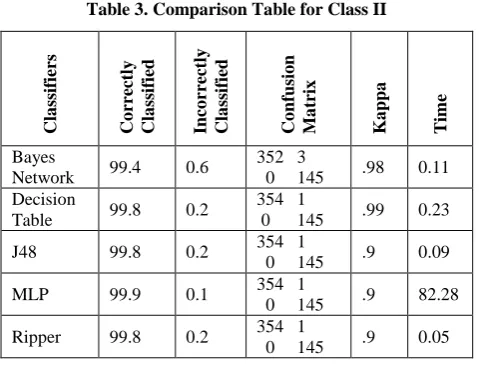
A glance at Table 3 reveals that (i) Of all the classifiers MLP algorithm is found to be very efficient and accurate. In this case the correctly classified instances are 99.9%, but the time complexity is more , (ii) In the case of Decision table, J48 and Ripper algorithms correctly classified instances are 99.8, but with regard to time complexity Ripper is preferred and with respect to Kappa statistics decision table is preferred, (iii) This is a two class problem in which the diagonal elements of the confusion matrix predicts the correctly classified instances, (iii) With regard to time complexity Ripper algorithm is found to be efficient, but the correctly
[image:3.595.310.550.116.305.2]classified instances are 99.8%. The values of error for each fold for class II is given in Table 4.
Table 3. Comparison Table for Class II
Cla
ss
ifi
er
s
Co
rr
ec
tly
Cla
ss
ifi
ed
Inco
rr
ec
tly
Cla
ss
ifi
ed
Co
n
fu
sio
n
Ma
tr
ix
K
a
p
p
a
Tim
e
Bayes
Network 99.4 0.6
352 3
0 145 .98 0.11 Decision
Table 99.8 0.2
354 1
0 145 .99 0.23
J48 99.8 0.2 354 1
0 145 .9 0.09
MLP 99.9 0.1 354 1
0 145 .9 82.28 Ripper 99.8 0.2 354 1
0 145 .9 0.05
Table 4. Values of error for each fold for Class II Folds Errors per
epoch Folds
Errors per epoch
1 .0000052 6 .0000095
2 .0000095 7 .0000054
3 .0000052 8 .0000095
4 .0000097 9 .0000050
5 .0000094 10 .0000057
Table 5. Comparison Table for Class III
Cla
ss
ifi
er
s
Co
rr
ec
tly
Cla
ss
ifi
ed
Inco
rr
ec
tly
Cla
ss
ifi
ed
Co
n
fu
sio
n
Ma
tr
ix
K
a
p
p
a
Tim
e
Bayes
Network 100 0
364 0
0 136 1 0.02 Decision
Table 100 0
364 0
0 136 1 0.2
J48 100 0 364 0
0 136 1 0.02
MLP 100 0 364 0
0 136 1 147.92
Ripper 100 0 364 0
0 136 1 0.02
5.3 Experiments on Class III
[image:3.595.47.287.199.483.2]Table 6. Values of error for each fold for Class III Folds Errors per
epoch
Folds Errors per epoch
1 .0000048 6 .0000091
2 .0000091 7 .0000048
3 .0000048 8 .0000091
4 .0000048 9 .0000091
5 .0000091 10 .0000048
5.4 Experiments on Class IV
[image:4.595.309.549.78.286.2]A glance at Table 7 reveals that (i) In this case, the correctly classified instances with respect to J48 and Ripper algorithms are 99.8%, as per kappa statistics Decision Table, J48 and Ripper are efficient (ii) This is a three class problem in which the diagonal elements of the confusion matrix predicts the correctly classified instances, (iii) With regard to time complexity , J48 is preferred. The value of errors for each fold is given in Table 8.
Table 7. Comparison Table for Class IV
C la ss if ie rs C o rr ec tl y C la ss if ie d In co rr ec tl y C la ss if ie d C o n fu si o n M a tr ix Ka p p a T im e Bayes
Network 94 6
331 24 0 0 90 0 0 6 49
.87 0.02
Decision
Table 99.6 0.4
355 0 0 0 90 0 2 0 53
.99 0.25
J48 99.8 0.2
354 0 0 0 90 0 2 0 55
.99 0.02
MLP 98 0.2
348 0 7 0 90 0 3 0 52
.95 96.13
Ripper 99.8 0.2
355 0 0 0 90 0 1 0 54
.99 0.05
Table 8. Values of error for each fold for Class IV
Folds Error per epoch Folds
Error per epoch
1 .0053658 6 .0053864
2 .0037565 7 .005319
3 .0048502 8 .0050499
4 .0034294 9 .0049518
5 .0051314 10 .0050978
5.5 Experiments on Class V
A glance at Table 9 reveals that (i) In this case, the correctly classified instances are 100% for all the classifiers except Bayes Network, Kappa statistics is 1 for all except Bayes Network, (ii) This is a two class problem in which the diagonal elements of the confusion matrix predicts the correctly classified instances, (iii) With regard to time complexity , J48 and Ripper algorithms are preferred. The value of errors for each fold is given in Table 10.
Table 9. Comparison Table for Class V
Cla ss ifi er s Co rr ec tly Cla ss ifi ed Inco rr ec tly Cla ss ifi ed Co n fu sio n Ma tr ix K a p p a Tim e Bayes
Network 98.2 1.8
413 9
0 78 .93 0.02 Decision
Table 100 0
422 0
0 78 1 0.27
J48 100 0 422 0
0 78 1 0.02
MLP 100 0 422 0
0 78 1 5.29
Ripper 100 0 422 0
[image:4.595.49.283.291.549.2]0 78 1 0.02
Table 10. Values of error for each fold Folds Error per
epoch Folds
Error per epoch
1 .0000093 6 .0000093
2 .0000093 7 .0000093
3 .0000093 8 .0000093
4 .0000093 9 .0000049
5 .0000093 10 .0000093
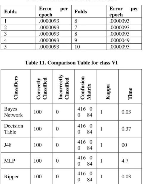
Table 11. Comparison Table for class VI
Cla ss ifi er s Co rr ec tly Cla ss ifi ed Inco rr ec tly Cla ss ifi ed Co n fu sio n Ma tr ix K a p p a Tim e Bayes
Network 100 0
416 0
0 84 1 0.03 Decision
Table 100 0
416 0
0 84 1 0.37
J48 100 0 416 0
0 84 1 00
MLP 100 0 416 0
0 84 1 4.7
Ripper 100 0 416 0
0 84 1 0.03
5.6 Experiments on Class VI
[image:4.595.309.549.307.617.2]Table 12. Values of error for each fold for Class VI
Folds Error per
epoch Folds
Error per epoch
1 .0000103 6 .0000135
2 .0000103 7 .0000103
3 .0000103 8 .0000103
4 .0000135 9 .0000056
5 .0000135 10 . 0000103
5.7 Experiments on Class VII
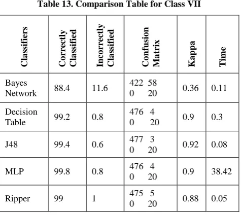
[image:5.595.50.291.85.177.2]A glance at Table 13 reveals that (i) In this case, the correctly classified instances are 99% fro Ripper and 99.8% for MLP, (ii) This is a two class problem in which the diagonal elements of the confusion matrix predicts the correctly classified instances, (iii) With regard to time complexity Ripper algorithm is found to be efficient. The Value of errors for each fold is given in Table 14.
Table 13. Comparison Table for Class VII
Cla
ss
ifi
er
s
Co
rr
ec
tly
Cla
ss
ifi
ed
Inco
rr
ec
tly
Cla
ss
ifi
ed
Co
n
fu
sio
n
Ma
tr
ix
K
a
p
p
a
Tim
e
Bayes
Network 88.4 11.6
422 58
0 20 0.36 0.11 Decision
Table 99.2 0.8
476 4
0 20 0.9 0.3
J48 99.4 0.6 477 3
0 20 0.92 0.08
MLP 99.8 0.8 476 4
0 20 0.9 38.42
Ripper 99 1 475 5
0 20 0.88 0.05
Table 14. Values of error for each fold for Class VII Folds Error per
epoch Folds
Error per epoch
1 .0000135 6 .0000146
2 .0000149 7 .0000149
3 .0000125 8 .0000149
4 .0000146 9 .000015
5 .0000138 10 . 0000148
5.8 Optimal Classifier for Class I to VII
The table 15 predicts the optimal classifier for the classes( I to VII) with regard to the different classifiers.Table 15. Accuracy of Different algorithms on Class I to VII
Cla
ss
es
Ba
y
es
Ne
two
rk
De
cisio
n
ta
b
le
J48 MLP Rip
p
er
I 95.6 96.7 92.7 98.7 98.9
II 99.4 99.8 99.8 99.8 99.8
III 100 100 100 100 100
IV 94.3 99.6 99.8 98 99.8
V 98.2 100 100 100 100
VI 100 100 100 100 100
VII 91.5 99.2 99.4 99.5 99.1
5.9 ROC
ROC curves depict the performance of a classifier without regard to class distribution or error costs. They plot the number of positives included in the sample on the vertical axis, expressed as a percentage of the total number of positives, against the number of negatives included in the sample, expressed as a percentage of the total number of negatives, on the horizontal axis.
[image:5.595.49.287.299.512.2]Table 16 gives the ROC values for various classes (I to VII) with respect to the classifiers considered here.
Table 16. ROC for Class I to Class VII
Cla
ss
es
Ba
y
es
Ne
two
rk
De
cisio
n
ta
b
le
J48 MLP Rip
p
er
I 99.1 98.4 87.3 99.5 98.9
II 100 99.8 99.9 99.8 99.9
III 100 100 100 100 100
IV 99.1 99.6 99.9 99.8 99.7
V 100 100 100 100 100
VI 100 100 100 100 100
VII 100 99.6 99.5 99.8 99.4
6.
CONCLUSION
[image:5.595.310.549.370.523.2]The results obtained from the present investigation using the data mining algorithms Bayes Network, J48, Decision table, MLP and Ripper on this data set for performance analysis are found to be highly accurate and hence the model is justified. It is amazing to note that almost all the DM algorithms have performed extremely well (with accuracy of 100%) on the data set generated and thus our model and approach are highly justified. This justifies the application of the methodology on State and National Level database. Any DM algorithm can be used for further analysis as the efficacy of the present analysis holds good for the macro Database also. The strength of analysis lies in its large scope of application.
As this model is designed using mathematical and computer based system, it is in a generalized form and the model can with minimum changes be adopted for any subject and can also be used in an integrated system to track overall progress of a child. The model because of its generic structure can be used across states and countries. Based on this Learning Model, a software using a DBMS and a Frontend can be developed for any hardware platform which can be used in schools or school administration hubs to track student progress and understand the learning curve in mathematics. The software can also be web enabled and integrated into the education sector of e-governance to share knowledge and information on mathematics learning across geographical boundaries. The progress tracking is an aid for diagnostic purposes in the areas of psychological counselling in counselling and medical centres and can be also used for
counselling and guidance in educational institutions. The Mathematical Pathway database and the Data Mining techniques can be further used to analyse learning trends which will be used by the decision makers at National or State level for making effective predictions to improve the quality of education. Finally it is concluded that the present methodology is unique and generic and can be extended to other disciplines.
7.
ACKNOWLEDGEMENT
One of us, Annapurna S Kamath is grateful to the Bangalore University for providing the research facilities to carry out the research program.
8.
REFERENCES
[1] Kamath, Annapurna, S., 2011. “Design and Development of a Learning Model to Optimize the Mathematical Pathway Using Mathematical Modeling and Computer Based Techniques”, Ph.D. Thesis, BU, India.
[2] Tan Pang-Ning et. al. 2006. Introduction to Data Mining. Pearson Education.
[3] Mucherino, A.,Papajorgji, P.J., Pardalos, P. 2009. Data Mining in Agriculture, Springer.
[4] Bhagyashree Ambulkar and Vaishali Borkar. 2012. Data Mining in Cloud Computing. IJCA Proceedings on National Conference on Recent Trends in Computing NCRTC(6):23-26, May 2012. Published by Foundation of Computer Science, New York, USA
[5] Li, J., Wong, L. and Yang, Q. 2005 . Data Mining in Bioinformatics, IEEE Intelligent System, IEEE Computer Society. Indian Journal of Computer Science and Engineering, Vol 1 No 2, 114-118
[6] Ankit Bhardwaj, Arvind Sharma, V.K. Shrivastava . 2012. Data Mining Techniques and Their Implementation in Blood Bank Sector –A Review. International Journal of Engineering Research and
Applications (IJERA) ISSN: 2248-9622 www.ijera.com Vol. 2, Issue4, July-August 2012, pp.1303-1309 [7] P. K. Srimani, Manjula Sanjay Koti. 2011.A Comparison
of different learning models used in Data Mining for Medical Data. 2nd International Conference on Methods and Models in Science and Technology (ICM2ST-11) Nov. 19-20, 2011, Maharani Palace, Jaipur, Rajasthan, India
[8] P. K. Srimani, Manjula Sanjay Koti. 2012. Outlier Mining in Medical Databases by using Statistical Methods. Engg. Journals Publication.
[9] Srimani et.al. 2012. Massive Data Mining(MDM) on Data streams using Clssification Algorithms. International Journal of Engineering Science and Technology (IJEST)Vol. 4 No.06 June 2012 pp 2839-2848
[10] Aubrey, D., 1996. “Mining for dollars,” Computer Shopper, Aug, 16-8, p. 568(3).
[11]Edelstein, H.,1996. “Mining data warehouses,” InformationWeek, Jan 08, 561, p. 48(4).
[12]Fausett, Laurene,1994. Fundamentals of Neural Networks: Architectures, Algorithms and Applications, Prentice-Hall, New Jersey, USA.
[13] Kosko, Bart,1992. Neural Networks and Fuzzy Systems, Prentice-Hall, New Jersey, USA.
[14]Sarle, Warren S.,1994. “Neural Networks and Statistical Models,” Proceedings of the Nineteenth Annual SAS Users Group International Conference, April, pp 1-13. [15] Heikki, Mannila, 1996. Data mining: machine learning,
statistics, and databases, IEEE.
[16] U. Fayadd, Piatesky, G. Shapiro, and P. Smyth, 1996. From data mining to knowledge discovery in databases, AAAI Press / The MIT Press, Massachusetts Institute Of Technology. ISBN 0–262 56097–6.
[17]Merceron, A., Yacef, K.. 2005 Educational Data Mining: a Case Study. In: Proceedings of the International Conference on Artificial Intelligence in Education (AIED2005), IOS Press,467--474 (2005).
[18]Q. A. Radaideh, E. W. Shawakfa, and M. I. AI-Najjar 2006. “Mining student data using decision trees”, International Arab Conference on Information Technology(ACIT'2006), Yarmouk University, Jordan [19]Romero, C., Ventura, S. 2007. Educational Data Mining:
A Survey from 1995 to 2005. Expert Systems with Applications 33, 125--146
[20] C. Romero, S. Ventura, E. Garcia.2008. "Data Mining in Course Management Systems: MOODLE Case Study and Tutorial". Computers & Education 51(1): 368–384. [21]Alaa el-Halees. 2009. “Mining students data to analyze
e-Learning behavior: A Case Study”,
[22] R. Baker, K. Yacef .2010. "The State of Educational Data Mining in 2009: A Review and Future Visions". Journal of Educational Data Mining, Volume 1, Issue 1
1: 3– 17.
[24]C. Romero, S. Ventura. 2010. Educational Data Mining: A Review of the State-of-the-Art. IEEE Transaction on Systems, Man, and Cybernetics, Part C: Applications and Reviews. 40(6), 601-618, 2010.
[25] Brijesh Kumar Baradwaj , Saurabh Pal. 2011. Mining Educational Data to Analyze Students‟ Performance, (IJACSA) International Journal of Advanced Computer Science and Applications, Vol. 2, No. 6, 2011, pp. 63-69 [26]U. K. Pandey, and S. Pal. 2010. “Data Mining: A
prediction of performer or underperformer using classification”, (IJCSIT) International Journal of Computer Science and Information Technology, Vol. 2(2), pp.686-690, ISSN: 0975-9646, 2011.
[27] Baker, R.S.J.d. 2011. Mining Data for Student Models. [28]B.K. Bharadwaj and S. Pal. 2011. “Data Mining: A
prediction for performance improvement using classification”, International Journal of Computer Science and Information Security (IJCSIS), Vol. 9, No. 4, pp. 136-140, 2011.
[29] Buckley, B. C., Gobert, J., Horwitz, P.2006. Using log files to track students' model-based inquiry. In: Proceedings of the 7th International Conference on Learning Sciences, 57—63.
[30]Srimani & Annapurna, 2012. “Neural Networks Approach for the Performance Analysis of the Learning Model – A Case Study, International Journal of Current Research, Vol4, Issue,04,pp236-239, April 2012.
[31]J. Han and M. Kamber,2006. “Data Mining: Concepts and Techniques,” Morgan Kaufmann.
[32]Adrians, p., and D.Zantiuge. 1996. Data mining.Harlow, England:Addison Wesley.
[33]David Heckerman. 1995. A tutorial on learning with Bayesian Networks.
[34]Ian H Witten, Eibe Frank. 2005. Data Mining :Practical machine learning tools and techniques. Second Edition, Morgan Kaufmann Publication.
[35]Becker, Barry G.,1998. Visualizing Decision Table Classifiers. Published in proceeding INFOVIS ‟98, Proceedings of the IEEE symposium on Information Visualization.
[36]Bigus, J. P. 1996. Data Mining with neural networks. New York:Mc.Grawhill.
[37]J. R. Quinlan,1986. “Introduction of decision tree: Machine learn”, 1: pp. 86-106.
[38]Quinlan, J. R., 1993. C4.5:Programs for Machine Learning. Morgan Kaufmann Publishers
[39]Spackman, K. A.,1989. Signal detection theory: Valuable tools for evaluating inductive learning. In Proceedings of the Sixth International Workshop on Machine Learning, pp. 160-163 San Mateo, CA. Morgan Kaufman.