The Geography of Knowledge Spillovers
between High-Technology Firms in
Europe. Evidence from a Spatial
Interaction Modelling Perspective
Fischer, Manfred M. and Scherngell, Thomas and
Jansenberger, Eva
Vienna University of Economics and Business, Vienna University of
Economics and Business, Vienna University of Economics and
Business
2005
The Geography of Knowledge Spillovers between High-Technology
Firms in Europe
Evidence from a Spatial Interaction Modelling Perspective
Manfred M. Fischer*+, Thomas Scherngell+ and Eva Jansenberger+
Institute for Economic Geography and GIScience
Vienna University of Economics and Business Administration, Austria
March 2005
*
Corresponding author, address for correspondence: Institute for Economic Geography and GIScience, Vienna University of Economics and Business Administration, Nordbergstr. 15, A-1090 Vienna.
+
Manfred M. Fischer is Professor and Chair of Economic Geography at Vienna University of Economics and Business Administration, Austria. Thomas Scherngell and Eva Jansenberger are research assistants at the same institution.
Abstract. The focus in this paper is on knowledge spillovers between high-technology
firms in Europe, as captured by patent citations. High-technology is defined to include the ISIC-sectors aerospace (ISIC 3845), electronics-telecommunication (ISIC 3832), computers and office equipment (ISIC 3825), and pharmaceuticals (ISIC 3522). The European coverage is given by patent applications at the European Patent Office that are assigned to high-technology firms located in the EU-25 member states (except Cyprus and Malta), the two accession countries Bulgaria and Romania, and Norway and Switzerland. By following the paper trail left by citations between these high-technology patents we adopt a Poisson spatial interaction modelling perspective to identify and measure spatial separation effects to interregional knowledge spillovers. In doing so we control for technological proximity between the regions, as geographical distance could be just proxying for technological proximity. The study produces prima facie evidence that geography matters. First, geographical distance has a significant impact on knowledge spillovers, and this effect is substantial. Second, national border effects are important and dominate geographical distance effects. Knowledge flows within European countries more easily than across. Not only geography, but also technological proximity matters. Interregional knowledge flows are industry specific and occur most often between regions located close to each other in technological space.
JEL Classification: O31, C21, R15, O52
Keywords: Knowledge spillovers, patent citations, high-technology, European regions,
1 Introduction
The last few years have witnessed an increasing interest in knowledge spillovers.
Knowledge spillovers1 may be defined to denote the benefits of knowledge to firms or individuals, not responsible for the original investment in the creation of this
knowledge. There are two distinct types of knowledge spillovers: Spillovers embodied
in traded capital or intermediate goods and services [so-called pecuniary externalities],
and spillovers of the disembodied kind [non-pecuniary externalities]. This paper
considers spillovers of the second type. Such spillovers arise when some of the R&D
activities have the classic characteristic of a non-rivalrous good and cannot be
appropriated entirely.
The importance of knowledge spillovers is widely recognised. Modern endogenous
growth theory, for example, casts knowledge spillovers from investments in R&D as a
central component in generating the increasing returns which sustain long-term growth
(see, for example, Romer 1990). In these theories, it is typically assumed that
knowledge spills over to other agents within the country, but not to other countries. Yet
there is no good reason to believe that knowledge stops spilling over because it hits a
national boundary.
The last few years have seen the development of a significant body of empirical
research on knowledge spillovers. Empirical analysis of the externalities is usually
carried out using the R&D expenditure that helps to create them, rather than the
inventions themselves. Many different measurements2 provide varied evidence of knowledge spillovers at the aggregate level. Most of the studies find some evidence for
1
In this paper we use the notions knowledge spillovers and knowledge externalities interchangeably.
2
such spillovers, some do not (see Griliches 1992, 1995). Generally speaking, this
research has shown that new technological knowledge spills over and complements
R&D in some industries, especially in high-technology ones (see Bernstein and Nadiri
1988).
But the spatial range of such knowledge spillovers is greatly contested3 (see Karlsson and Manduchi 2001). Several explanations have been offered for this lack of agreement,
such as for example the notorious difficulty to measure knowledge spillovers. Indeed,
Krugman (1991, p. 53) has argued that economists should abandon any attempts at
measuring knowledge spillovers because "knowledge flows ... are invisible; they leave
no paper trail by which they may be measured and tracked". The work of Jaffe,
Trajtenberg and Henderson (1993), however, pointed to one important exception. They
argued that spillovers of knowledge may well leave a paper trail in the citations to
previous patents recorded in patent documents. Because patent documents contain
detailed information about the technology of the patented invention, the inventor and
his/her residence, the assignee (generally, the firm) that owns the patent rights, and
citations to previous patents, these patent documents provide an important resource for
analysing the geography of knowledge spillovers.
This paper follows Jaffe, Trajtenberg and Henderson (1993) to use patent citations as a
proxy for knowledge spillovers4. The focus is on externalities within the
3
Most studies identifying the spatial extent of knowledge spillovers are based on the Griliches-Jaffe knowledge production function model to measure knowledge spillovers, indirectly via effects on the output of the knowledge production function. Note, however, that this type of research is not without problems. The problems center around the question of whether the spatial units of observation are appropriately chosen, whether and how spatial effects are taken into account, how the output of the knowledge production process is measured, whether available measures actually capture the contribution of R&D spilled-over, how the spillover pools are constructed, and R&D capital deflated and depreciated. Despite these difficulties, there has been a significant number of reasonably well done studies (see, for example, Anselin, Varga and Acs 1997; Bottazzi and Peri 2003; Fischer and Varga 2003), all pointing in the direction that knowledge spillovers tend to be geographically bounded within the region of knowledge production.
4
technology sector5. The objective of the paper is to identify and measure those types of spatial separation that tend to impede the likelihood of knowledge spillovers between
regions in Europe6. In particular, we are interested in the questions whether or not knowledge – as captured by patented inventions – flows more easily within countries
than between, and to what extent geographic distance between inventions has an
influence on these knowledge flows. As we consider spatial separation effects to
interregional spillovers in a multiregional setting it is important to control for
technological proximity between regions as geographical distance could be just
proxying for technological proximity.
In using patent citation data from the European Patent Office [EPO] this paper builds on
recent work by Maurseth and Verspagen (2002), but departs from this prior analysis in
four major aspects. First, it adopts a spatial interaction modelling perspective to identify and measure spatial separation effects, and develops the appropriate model specification
to account for the integer nature of interactions in the given context. Second, we follow the paper trail left by individual patent citations in high-technology industries to track
the individual flows within a discrete representation of space. This allows us to properly
control for intrafirm patent citations7. Third, citations to a patent are counted for a window of five years to overcome at least partially the truncation bias that is due to the
fact that we observe citations for only a portion of the life of an invention, with the
duration of that portion varying across patent cohorts. Finally, the study extends the geographic coverage, essentially from the EU-15 to the EU-25 countries on the one
side, and limits the context to the high-technology sector on the other.
The reminder of the paper is organised as follows. The section that follows explains in
some more detail the nature of patents and patent citations, and briefly discusses how
patent citations can be used as an indicator for knowledge spillovers. Section 3
5
Following Hatzichronoglou (1997) we define high-technology to include the ISIC-sectors pharmaceuticals (ISIC 3522), computers and office equipment (ISIC 3825), electronics-telecommunication (ISIC 3832), and aerospace (ISIC 3845).
6
We have chosen 188 regions (see Appendix A) that cover the EU-25 member countries (except Cyprus and Malta), the accession countries Bulgaria and Romania, and Norway and Switzerland.
7
elaborates on the patent citation data to be used in the study. In Section 4, we outline the
spatial interaction modelling framework that is pertinent to the model development in
this study. Section 5 develops a Poisson model specification that accommodates the true
integer nature of patent citation flows and derives maximum likelihood estimates of the
model parameters. Section 6 generalises this model specification to allow for the
overdispersion in the data by letting each pair's of regions Poisson parameter have a
random distribution of its own. In Section 7 we present the estimation results of the
basic Poisson spatial interaction model and its generalisation. We conclude with a
summary and evaluation of our results in the final section.
2 Patents, Patent Citations and Knowledge Spillovers
A patent is a property right awarded to inventions for the commercial use of a newly
invented device. An invention to be patented has to satisfy three patentability criteria. It
has to be novel and non-trivial in the sense that it would not appear obvious8 to a skilled practitioner of the relevant technology, and it has to be useful, in the sense that it has potential commercial value. If a patent is granted, an extensive public document is
created. The document contains detailed information about the invention, the inventor,
the assignee, and the technological antecedents of the invention. Because patents record
the residence of the inventors they are an invaluable resource for studying how
knowledge flows are affected by geography.
Patent related data, however, have two important limitations9. First, the range of patentable inventions constitutes only a subset of all R&D outcomes, and second, patenting is a strategic decision and, thus, not all patentable inventions are actually
patented. As to the first limitation, purely scientific advances devoid of immediate
applicability as well as incremental technological improvements which are too trite to
pass for discrete, codifiable inventions are not patentable. The second limitation is
8
What is obvious or not can be very difficult to evaluate. Different national patent offices have taken different approaches to this problem. While, for example, among the European countries, in Germany the threshold is comparatively high, the requirements in the UK are much lower. In extreme cases, this may lead to a situation where a patent on a given subject is granted in one country, but not in another (Michel and Bettels 2001).
9
rooted in the fact that it may be optimal for inventors not to apply for patents even though their inventions would satisfy the criteria for patentability (Trajtenberg 2001).
Inventors balance the time and expense of the patent process, and the possible loss of
secrecy which results from patent publication, against the protection that a patent
potentially provides to the inventor10 (Jaffe 2000). Therefore, patentability requirements and incentives to refrain from patenting limit the scope of our analysis based on patent
data.
Patent citations capture only those spillovers which occur between patented pieces of an
invention, and, thus, underestimate the actual extent of knowledge spillovers. Other
channels of knowledge transfers are not captured by patent citations, such as, for
example, interfirm transfer of knowledge embodied in skilled labour; knowledge flows
between customers and suppliers; knowledge exchange at conferences and trade fairs,
etc. Thus, our study refers only to a very specific and limited form of interfirm
knowledge flows.
It is also clear that patent citations not always represent what we typically think of as
knowledge spillovers. Some citations may represent noise11. This is certainly the case for citations added by the patent examiner of which the citing inventor was unaware.
This noise creates a bias against finding spillovers. Fortunately, Thompson (2003)
illustrates that bias in this direction is a problem of power, which can be overcome with
a sufficiently large sample size. His result also implies that patent citations are more
indicative of patterns of knowledge flows at the level of organisations, industries and
regions than at the level of individual patents (Jaffe, Fogarty and Banks 1998).
3 The Patent Citation Data and Some Descriptive Statistics
10
Though some firms may choose not to patent inventions, patenting in high-technology industries is commonly practiced and a vital part of maintaining technological competitiveness. High-tech firms use patents not only to protect the returns to specific inventions but also to block products of their competitors, as bargaining chips in cross-licensing negotiations, and/or to prevent or defend against infringement suits (Jaffe 2000, Almeida 1996).
11
The European coverage in our study is achieved via European patent applications. By
European patent applications we mean patents applied at the European Patent Office [EPO]12 and assigned to organisations located in the EU-25 member states [except Cyprus and Malta], the two accession countries Bulgaria and Romania, and Norway and
Switzerland. Our data source is the European Patent Office [EPO] database. This is a
natural choice for the purpose of our study because patents from different national
patent offices are not comparable to each other. There are different patenting costs,
approval requirements, citation practices and enforcement rules across Europe.
The focus is on corporate patents in the high-technology sector. We used MERIT's
concordance table (Verspagen, Moergastel and Slabbers 1994) between the four-digit
ISIC-sectors and the 628 patent subclasses of the International Patent Code (IPC)
classification13 to identify such patents from the universe of European patent applications. Our core data set includes all the high-technology patents with an
application date in the years 1985-2002, totalling 177,424 patents. Data on the inventor
and his/her location, the assignee [that is, the legal entity that owns the patent rights,
assigned to it by the inventor(s)], the time of application, the technology of the
invention as captured by IPC codes, and EPO patent citations are the main pieces of
information used from this file. We selected corporate patents, that is, patents assigned
to non-government organisations located in Europe, since our interest is on interfirm
research spillovers.
Patent citation is a phenomenon that derives from the relationship between two
inventions or inventors as evidenced by a citing patent and a cited patent. The data on
12
Patent protection in Europe can be obtained by filing national applications and European applications. This implies that patent data from the European Patent Office do cover only a subsample of patents applied for in Europe.
13
this relationship come in form of citations made [that is, each patent lists references to previous patents]. For identifying the citation flows we need a list of cited and citing
patent applications. This requires in fact access to all citation data in a way that permits
efficient search and extraction of citations not by the patent number of the citing patent
but by the patent number of the cited patent.
While previous work indicates the usefulness of patent citations as an indicator for
aggregate knowledge flows, it also highlights the need for careful attention to various
biases that make their interpretation risky. In particular, the observation of citations is
subject to a truncation bias because we observe citations for only a portion of the life of
an invention, with the duration of that portion varying across patent cohorts. This means
that patents of different ages are subject to different degreesof truncation. To overcome
this problem at least in part we have identified all the pairs of cited and citing patents
where citations to a patent are counted for a window of five years following its issuance.
The analysis is, thus, confined to 1985-1997 in the case of cited patents while citing
patents appearing in 1990-2002 are taken into account. Although the five-year horizon
appears to be short, it does capture a significant amount of a typical patent's citation
life14.
Given our interest on pure externalities (that is, on interfirm knowledge spillovers),
citations to patents that belong to the same assignee [so-called self-citations] were
eliminated, resulting into 98,191 interfirm patent citations15. The elimination of self-citations – in this and all prior work – remains far from satisfactory. Although we have
manually checked the sample for cases where company names are sufficiently similar to
identify self-citations between parents and their subsidiaries, and joint ventures, this
effect can only get us so far. One could presumably complete the process using
directories of company ownership (such as Dun & Bradstreet's Who owns Whom). But,
14
The mean citation lag of all citations in 1985-2002 is 4.62 years, with some sectoral differences: pharmaceuticals (4.4 years), computers and office equipment (4.4 years), electronics-telecommunication (4.7 years) and aerospace (5.4 years).
15
daunting as that task would be, one must then decide when a citation is a self-citation
and when it represents a spillover. The judgement depends on the degree of interaction
taking place between related firms. This does not seem to be an operational criterion
(Thompson 2003).
The spatial interaction modelling perspective we adopt in this study shifts attention
from individual patent citations to interregional patent citations or from the dyad "cited
patent – citing patent" to the dyad "cited region – citing region". Accordingly, all
citation data were aggregated into a region-by-region matrix (cij) where cij denotes the
number of patent citations from region j (j=1, ..., J) to region i (i=1, ..., I). The rows of the matrix represent the regions of the cited patents [that is, the origins of spillovers]
and the columns the regions of the citing patents [that is, the spillover absorbing
regions]. The matrix is asymmetric in nature, that is, cij≠cji.
We have chosen I=J=188 regions, generally NUTS-2 regions for the EU-15 countries16 and NUTS-0 regions for the other countries. NUTS is an acronym of the French for the
'nomenclature of the territorial units for statistics', which is a hierarchical system of
regions used by the statistical office of the European Community for the production of
regional statistics. At the top of the hierarchy are the NUTS-0 regions (countries), below
which are NUTS-1 regions (regions within countries) and then NUTS-2 regions
(subdivisions of NUTS-1 regions).
In the case of cross-regional inventor-teams we have used the procedure of multiple full
counting17. This procedure deviates from the USPTO [United States Patent and Trademark Office] practice to select first-named addresses only18. In order to clarify the difference between the two assignment procedures let us assume that patent A with three inventors in three different regions – say i, j and k – cites patent B with two inventors in two different regions, say s and t. In this case the USPTO practice would count only the
16
In some cases (Denmark, Greece, Ireland and Luxembourg) NUTS-0 regions are used as dictated by practical convenience. Details of the regional system are given in Appendix A.
17
Note that full rather than fractional counting does justice to the true integer nature of patent citations, but gives the interregional cooperative inventions greater weight.
18
cross-regional citation link Ai to Bs, while our procedure takes all six patent citation
links into account. Evidently, the USPTO procedure underestimates, our method
overestimates knowledge spillovers.
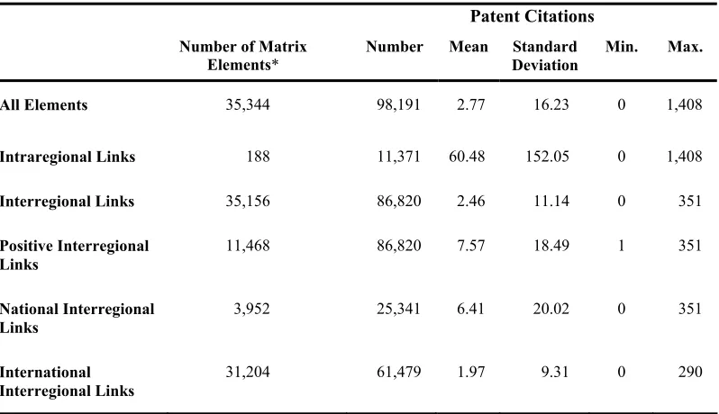
Table 1: Descriptive Statistics on the Region-by-Region Citation Matrix
Patent Citations
Number of Matrix Elements*
Number Mean Standard Deviation
Min. Max.
All Elements 35,344 98,191 2.77 16.23 0 1,408
Intraregional Links 188 11,371 60.48 152.05 0 1,408
Interregional Links 35,156 86,820 2.46 11.14 0 351
Positive Interregional Links
11,468 86,820 7.57 18.49 1 351
National Interregional Links
3,952 25,341 6.41 20.02 0 351
International Interregional Links
31,204 61,479 1.97 9.31 0 290
* Elements of the region-by-region citation matrix
Table 1 provides some basic information about the region-by-region citation matrix.
The (188, 188)-matrix contains 35,344 elements with a total of 98,191 citations between
high-technology firms. The mean number of citations between any two regions
(including intraregional flows) is 2.77, but the standard deviation is rather high.
Interregional citations show a highly skewed distribution. About two thirds of all pairs
(i, j; i≠j) of regions [23,688 pairs] never cite each other's patents. The frequency of patent citations gradually declines for more intensive citation links. There are only 90
pairs of regions for which the number of citations is 100 or more. The average number
of citations for all interregional pairs is 2.46 and the average for those that cite each
other 7.57. Table 1 indicates that national patent citations are more frequent than
[image:11.595.91.490.193.423.2]4 The Spatial Interaction Modelling Perspective
We adopt a spatial interaction modelling perspective to identify and measure spatial
separation effects to interregional knowledge spillovers as captured by patent citations
among high-technology firms. Mathematically, the situation we are considering is one
of observations cij (i=1, ..., I=188; j=1, ..., J=188) on random variables, say Cij, each of
which corresponds to the interfirm transfer of knowledge from region i to region j. We are interested in models of the type
ij ij ij
C =µ ε+ i=1, ..., I; j=1, ..., J; i≠j (1)
where the observed patent citation flows cij are independent Poisson variates with
[ ]
ij E Cij
µ = . The error εij is noise, with the property E[εij|cij]=0 by construction.
Note that this error term relates to a pair (i, j) of regions. We aim to develop appropriate models for the systematic part, µij, of the stochastic relationship with other random
variables which are the forecasts.
Spatial interaction models simultaneously incorporate the effect of origin and
destination characteristics and separation. Mathematically, they may be written as
( )
ij A B F di j ij ij
µ = i=1, ..., I; j=1, ..., J; i≠j (2)
where µij denotes the estimated knowledge flow from region i to region j. Ai represents
a factor characterising the origin i of interaction, and Bj a factor characterising the
destination j of interaction, while Fij is a factor that measures separation from i to j.
Origin and destination factors may be viewed as weights associated with origin and
destination variables. Their classical specifications are given by power functions
1
1
( , )
i i i
A = A a α =aα i=1, ..., I (3)
2
2
( , )
j j j
where α1 and α2 are parameters to be estimated and ai and bj denote some appropriate
origin and destination variables. The product Ai Bj in (2) can be interpreted simply as the
number of distinct (i, j)-interactions which are possible. In the current study ai is
measured in terms of the number of patents in the knowledge producing region i in the time period 1985-1997, and bj in terms of the number of patents in the knowledge
absorbing region j in the time period 1990-2002.
The separation function Fij constitutes the very core of spatial interaction models.
Hence, a number of alternative specifications of Fij have been proposed. In this study
we use the multivariate separation function
( )
1
( , ) exp
K
k
ij ij k ij
k
F F d β d
=
= =
∑
β i=1, ..., I; j=1, ..., J; i≠j (5)
that provides a flexible representational framework for the purpose of our study.
(1) ( )
( , ..., K )
ij ij ij
d = d d denotes the K separation measures. βk (k=1, ..., K) are unknown parameters.
Our interest is focused on K=4 measures: dij(1)represents geographic distance measured in terms of the great circle distance [in km] between the regions’ economic centres, dij(2)
is a dummy variable19 that represents border effects measured in terms of the existence of country borders between i and j, while dij(3) is a dummy variable20 that represents language barrier effects. As we consider the distance effect on interregional patent
citations it is important to control for technological proximity between regions, as
geographical distance could be just proxying for technological proximity. To do this we
use the technological proximity index sij developed by Maurseth and Verspagen (2002).
We divide the high-technology patents into fifty-five technological subclasses,
19
The dummy is set equal to zero for pairs of regions that are located within the same country, and to one otherwise.
20
following the International Patent Code (IPC) classification. Each region is then
assigned a (55, 1)-'technology vector' that measures the share of patenting in each of the
technological subclasses for the region. The technological proximity between two
regions i and j is given by the uncentred correlation of their technological vectors. Two regions that patent exactly in the same proportion in each subclass have an index equal
to one, while two regions patenting only in different subclasses have an index equal to
zero. This index is appealing because it allows for a continuous measure of
technological distance, namely (4)
1
ij ij
d = −s , and avoids the problem of defining
technological distance between sectors.
Integrating (2)-(5) into (1) yields
1 2 ( )
1
exp
K
k
ij i j k ij ij
k
C a bα α β d ε
=
= +
∑
i=1, ..., I; j=1, ..., J; i≠j. (6)Fitting this model to the patent citation data is a question of estimating the unknown
parameters α α1, 2 and βk (k=1, ..., K). At a first glance it is tempting to express (6)
equivalently as a log-additive model of the form
( )
1 2
1
log log log
K k
ij i j k ij ij
k
C α a α b β d u
=
= + +
∑
+ i=1, ..., I; j=1, ..., J; i≠j (7)with
(
2)
0,u∼N σ (8)
and then proceed to estimate the parameters by ordinary least squares regression of the
observations cij on ai, bj, and dij.
antilogarithms of these estimates are biased estimates of µij. One of the effects of this is
to underpredict large patent citations flows, and to underpredict the total flow (see
Flowerdew and Aitkin 1982). Second, estimating the parameters by the ordinary log-additive regression model given by Equations (7)-(8) would only be justified
statistically if we believed that flows Cij were independent and log-normally distributed
about their mean value with a constant variance. Such an assumption, however, is not
valid since patent citation flows are discrete counts whose variance is very likely to be
proportional to their mean value (see Bailey and Gatrell 1995, among others).
5 The Poisson Model Specification and Maximum Likelihood
Estimation
Least squares and normality assumptions ignore the true integer nature of patent citation
flows and approximate a discrete-valued process by an almost certainly
misrepresentative continuous distribution (Fischer and Reismann 2002). To overcome
this deficiency, it seems natural to assume that the Cij given Ai, Bj and Fij are iid Poisson
distributed with density
( )
exp , ,
!
ij
c ij ij
ij ij i j ij
ij
f C c A B F
c
µ µ
−
= =
(9)
where the mean parameter µ [that is, the conditional expectation of (i, j) patent citations, given Ai, Bj, Fij] is parameterised as
(
)
1 2
, , exp log ( , ) log ( , ) log ,
ij i j ij i j ij
E c A B F = A a α + B b α + F d β (10)
with dij =(dij(1),...,dij(K)) and β =(β1, ...,βK). Specification (10) is called the
exponential mean function21. The model comprising (9) and (10) is referred to as the
21
The parameter
1 2 1
( , , , ..., )
K
basic Poisson model specification. Note that µij is a deterministic function of Ai, Bj and
Fij, and the randomness in the model comes from the Poisson specification of cij.
Parameterisation (10) implies a particular form of heteroskedasticity, due to
equidispersion or equality of conditional variance and conditional mean:
, , , , .
ij i j ij ij i j ij ij
V c A B F =E c A B F =µ (11)
It also implies the conditional mean to have a multiplicative form given by
1 2
1 2
, , exp log ( , ) log ( , ) log ( , )
( , ) ( , ) ( , ).
ij i j ij i j ij
i j ij
E c A B F A a B b F d
A a B b F d
α α
α α
= + + =
=
β
β (12)
The Poisson specification of the spatial interaction model (6) shows some interesting
advantages. First, it is analogous to the familiar econometric regression specification (7)-(8) in many ways. In particular, E c A B ij i, j, Fij=µij. Moreover, parameter estimation is straightforward and may be done by maximum likelihood. Second, the 'zero problem', cij=0, is a natural outcome of the Poisson specification. In contrast to the
logarithmic regression specification there is no need to truncate an arbitrary continuous
distribution. The integer property of the outcomes cij is handled directly.
Parameter Estimation
For notational economy, let us denote θ the (K+2)-dimensional parameter vector
(
α α β1, 2, 1, ...,βK)
=(α α1, 2, )β that has to be estimated. The standard estimator for themodel is the maximum likelihood estimator. The likelihood principle selects as
estimator of θ the value which maximises the joint probability of observing the sample
values cij. This probability, viewed as a function of parameters conditional on the data,
1 1 1
( ) , , ,
I J
ij i j ij
i j
j
Lθ f c A B F
= =
≠
=
∏∏
θ (13)where we suppress the dependence L(θ) on the data and have assumed independence over (i, j). Maximising L(θ) is equivalent to maximising the log-likelihood function (see Sen and Smith 1995)
{
}
1 2
1 1
1 2
1 2 1
1 1 1
( ) 2
1
( ) log ( ) ( , ) ( , ) exp[ ]
[log ( , ) log ( , ) ) ] log ( !)
{ ( , ) ( , ) exp( )} log ( , )
log ( , )
I J
i j ij
i j
j ì
ij i j ij ij
I J I
i j ij i i
i j i
j ì
J
k
j j k ij ij
j j ì
L A a B b d
c A a B b d c
A a B b d c A a
c B b d c
α α
α α
α α α
α β = = ≠ • = = = ≠ • = ≠ = = − + + + + − = = − + + + +
∑ ∑
∑ ∑
∑
∑
θ θ β
β β
L
1 1 1
log ( !)
K I J
ij
k i j
j ì c = = = ≠ −
∑
∑ ∑
(14)where ci• =
∑
Jj=1cijand 1 Ij i ij
c• =
∑
= c .The partial derivatives of L(θ) are:( )
[
]
2 1 1 1 1 1( , ) exp
( , )
( , ) for 1,...,
J
ij
j ij
j i
i i i
c
B b d
A a
c A a i I
ϑ α ϑα α µ α = − • • = − + = = − =
∑
θ β L (15)( )
1 1 2 2 1 2( , ) exp
( , )
( , ) for 1,...,
I
ij
i ij
i j
j j j
c
A a d
B b
c B b j J
ϑ α ϑα α µ α = − • • = − + = = − =
∑
θ β L (16)( )
{
( ) ( )}
1 2 1 1 ( ) 1 1( , ) ( , ) exp
for 1,...,
I J
k k
ij i j ij ij ij
i j
k
j ì
I J
k
ij ij ij
i j
j ì
d A a B b d c d
d c k K
ϑ α α
with µi• =
∑
Jj=1µij and 1 Ij i ij
µ• =
∑
= µ . Maximum likelihood estimates may be found bymaximising L
( )
θ directly using iterative procedures, usually gradient algorithms, such as Newton-Raphson. Alternatively, one could set the partial derivatives of L( )
θ [that is, Equations (15), (16) and (17)] equal to zero and solve the resultant equations:( ) ( )
1 1 1 1
for =1, ..., and for =1, ..., , and
for 1,..., .
i i j j
I J I J
k k
ij ij ij ij
i j i j
j ì j ì
c i I c j J
d d c k K
µ µ
µ
• • • •
= = = =
≠ ≠
= =
= =
∑ ∑
∑ ∑
(18)Convergence is guaranteed because the log-likelihood function is globally concave22.
6 A Generalisation of the Poisson Spatial Interaction Model
The above Poisson model specification does not allow for individual (i, j)-effects, given the exogenous variables Ai, Bi, Fij. The exogenous variables are assumed to summarise
all individual deviations. Also, it is clear that the existence of fixed effects at the
individual level of (i,j) pairs is likely to exist in interregional patent citation relationships. This individual effect problem can be partly solved23 by introducing a heterogeneity term in the mean µij of the Poisson distribution such that the
multiplicative heterogeneity term exp(ξij) follows a gamma distribution with mean one
and variance δ:
*
Poisson ( )
ij ij
c ∼ µ (19)
where
22
The Hessian of the log-likelihood function is always negative. After estimation, the negative inverse of the estimated Hessian can be used for estimation of the asymptotic covariance matrix of the parameter estimates.
23
*
1 2
1 2
exp log ( , ) log ( , ) log ( , )
exp log ( , ) log ( , ) log ( , ) exp( )
ij i j ij ij
i j ij ij
A a B b F d
A a B b F d
µ α α ξ
α α ξ
= + + + =
= + +
β
β (20)
and
1
exp(ξij)∼Gamma (δ δ− , ). (21)
If exp(ξij) is gamma distributed and independent of the explanatory variables, cij has a
negative binomial distribution (Cameron and Trivedi 1998):
1
1 1
1 1 1
( )
, , ,
( 1) ( )
ij
c
ij ij
ij ij i j ij
ij ij ij
c f C c A B F
c
δ
Γ δ δ µ
δ
Γ Γ δ µ δ µ δ
− − − − − − + = = + + +
(22)
where Γ(.) is the gamma function and δ ≥0 the dispersion parameter. The larger δ is,
the greater the dispersion. Specification (22) with (20)-(21) is referred to as the
heterogeneous Poisson model of interregional patent citations. This modification leaves the mean unchanged, but changes the variance to
{
*} {
*}
* *( )ij ( ij | ij) ( ij| ij) ( ij) ( ij) ij(1 ij).
V c =E V c µ +V E c µ =E µ +V µ =µ +δ µ (23)
Thus, the model allows for overdispersion (that is, δ >0), with δ =0 reducing to the basic Poisson specification (9)-(10).
Estimation of the model may proceed with maximum likelihood. The log-likelihood
function is
{
}
}
1 1 1 1 1 1 2 1 2 ( )( , ) log log !
( )
( ) log 1 exp ( , ) ( , ) ( , )
log log ( , ) ( , ) ( , ) .
I J
ij
ij
i j
j ì
ij i j ij
ij ij ij i j ij
c
c
c A a B b F d
c c c A a B b F d
Γ δ
δ
Γ δ
δ δ α α
δ δ α α
7 Estimation
Results
Table 2 reports the results from the estimation of the two Poisson spatial interaction
model specifications [see Equations (9) and (10), and equation (22) with (20) and (21),
respectively] by maximum likelihood, using Newton-Raphson. The maximum
likelihood estimates of the basic Poisson spatial interaction model specification are
given in the first column, those of the generalised Poisson model in the second.
Standard errors are presented in brackets rather than t-statistics to allow comparison with the precision of the negative binomial maximum likelihood estimates in the second
column. The reported standard errors all assume correct specification of the variance
function. They are characterised by low significance levels.
Table 2: Estimation Results of the Poisson Spatial Interaction Model Specifications
[N=35,156 observations; asymptotic standard errors in brackets]
Poisson Spatial Interaction Model Variable
without Heterogeneity with Heterogeneity
Log-Likelihood -51,801.10 -37,235.05
{Corr (cij, predicted cij)}2
Wald Chi-Square (6)
0.686
307,522.81
0.783
30,552.12
Independent Variables
Origin Variable [α1] 0.833
***
(0.002)
0.915*** (0.006)
Destination Variable [α2] 0.858
***
(0.002)
0.885*** (0.006)
Geographical Distance [ß1]
Country Border [ß2]
Language Barrier[ß3]
Technological Proximity [ß4]
-0.270*** (0.005) -0.050*** (0.007) -0.238*** (0.014) 0.928*** (0.032) -0.321*** (0.014) -0.533*** (0.046) -0.031*** (0.043) 1.219*** (0.130)
Intercept -10.278*** (0.051)
-10.881*** (0.124)
Dispersion Parameter (δ) – 0.725
(0.014 )
Note: All independent metric variables are expressed as natural logs in order to lessen the impact of outliers. The origin, destination and separation functions are specified as follows: 1
( i, i) i
Aa α =aα ,
2 2
( ,j ) j
B b α =bα and ( )
1
( , ) exp ( K k )
ij k ij k
F d d β
=
=
∑
[image:20.595.84.510.370.701.2]the cited region i, bj in terms of patents (1985-2002) in the citing region j,
(1)
ij
d representing geographic distance is measured in terms of the great circle distance [km] between the economic centres in i and j;
( 2 )
ij
d is a dummy that represents border effects [zero for pairs (i, j) that are located in the same country,
one otherwise], dij( 3) is a dummy that represents language barrier effects [zero for pairs (i, j) that share the same language, one otherwise]; dij( 4 ) =1−sij where sij denotes technological proximity of regions i and j in a 55-dimensional technology space; *** denotes significance at the one percent level.
The estimated value of the dispersion parameter δ indicates that the basic Poisson model
specification has to be rejected [H0: δ =0, G2 =29,256.6, p<0.01]24. The rejection of this
model version is due to the situation of overdispersion which is associated with
unobserved heterogeneity among (i, j) pairs of regions. Therefore, the Poisson model specification with heterogeneity is preferred. The variance-mean equality assumption of
the Poisson model is too restrictive to adequately describe the patent citation flows.
The parameters of the negative binomial distribution are estimated along with a large
increase in the log-likelihood function compared to the Poisson model. The negative
binomial parameter estimates are generally somewhat larger in magnitude than the basic
Poisson ones, with the exception of the language dummy. But, since the negative
binomial specification allows for an additional source of variance, the estimated
standard errors are all larger, and therefore the conclusions to be drawn, while similar to
those derived from the basic Poisson model specification, are less precise.
The Poisson spatial interaction model specification with heterogeneity yields highly
significant effects. Both α-estimates are – in accordance with expectations – close to
one25. Geographical distance between inventors has a strong and negative effect on the likelihood of high-technology patent citations. The parameter estimate, βˆ1= −0.321,
24
The G-squared statistic is defined to be 1
1 1
ˆ ˆ
log( ) ( )
[ ]
{ }
I J
ij ij
ij ij ij
i j j ì
c c µ− c µ
= = ≠
− −
∑∑
where (cij logcij) = 0 if cij= 0(see Bishop, Fienberg and Holland 1975).
25
indicates that for any additional 100 km between regions i and j the (i, j)-mean patent citation frequency decreases by 27.5 percent. This suggests spillovers between
high-technology firms are impeded by geographical distance.
Not only distance, but also border effects matter. The point estimate of the coefficient β2
is nearly twice times as large as that of β1, showing that border effects are more
important than distance effects. Citing patents are much more likely to come from the
same country as the cited patents. High-technology related knowledge flows much more
easily within than between countries. This is a finding that corresponds well with the
notion of national systems of innovation26. Note that language barriers though significant have only a rather small effect (βˆ3 =–0.031) on interregional knowledge
spillovers.
The variable technological proximity controls for spillovers that are stronger between
technologically similar regions. The point estimate for the variable shows an effect that
is about four times larger than the distance effect even though the estimate is not very
precise. Interregional patent citation flows tend to follow particular technological
trajectories as defined at the three-digit level of the IPC classification. This indicates
that patent citation flows are industry specific and occur most often between regions not
too far located from each other in technological space. Technological proximity matters
more than geographical proximity.
8 Summary and Conclusions
A revival of interest in economic geography during the last decade has renewed efforts
to consider knowledge spillovers as a geographical phenomenon. In adopting this view
one is confronted with two challenges. The first is the notoriously difficult issue to
measure knowledge spillovers and the second one the issue to model the geographic
dimension of knowledge spillovers. In confronting the first challenge we used patent
citations as proxy for knowledge spillovers and followed the paper trail left by patent
26
citations to track this specific type of knowledge flows within the high-technology
sector across Europe. To address the second challenge we adopted a spatial interaction
modelling perspective. This perspective shifted the focus of attention from individual to
interregional patent citations, from the dyad "cited patent – citing patent" to the dyad
"cited region – citing region".
The basic goal of this study has been to identify and measure spatial separation effects
to interregional knowledge spillovers. In particular interest was focused on the
following three questions: To what extent geographical distance has an impact on
interregional knowledge spillovers? How important are national border effects as
distinct from geographical distance? Do linguistic borders matter? We have used a
Poisson spatial interaction model specification with heterogeneity to address these
questions. It is important to note that in doing so we have controlled for technological
proximity between regions, as geographical distance could be just proxying for
technological proximity.
The previous section has produced prima facie evidence that knowledge spillovers are
geographically localised. National borders have a negative impact on knowledge flows,
and this effect is very substantial. Knowledge flows are larger within countries than
between regions located in different countries. The results also indicate that
geographical proximity matters, while also suggesting that these effects are much
smaller than the border effects. Knowledge spillovers occur more often between regions
that belong to the same country and are in geographical proximity. Technology
proximity tends to overcome geographical proximity. Interregional knowledge flows
seem to follow particular technological trajectories, and occur most often between
regions that are located in technological space, not too far from each other.
The results support the conclusion that national and sectoral systems of innovation
matter at least as far as high-technology firms are concerned. This is a conclusion that
has important policy implications. European regional cohesion appears to be at stake,
especially – but not exclusively – because of the localised nature of knowledge flows.
The results also have important implications for modelling technological change and
economic growth, such as Romer (1990), in which localised knowledge spillovers are
simply assumed.
Acknowledgement: The authors gratefully acknowledge the grant no. 11329 provided by the Jubiläumsfonds of the Austrian National Bank. The authors are also grateful to Bernd Bettels (EPO) for supplying the data and to Katarina Kobesova (Institute for Economic Geography and GIScience) for developing the patent citation database.
References
Almeida, P. (1996). "Knowledge Sourcing by Foreign Multinationals: Patent Citation Analysis in the U.S. Semiconductor Industry." Strategic Management Journal 17, 155-65.
Bailey, T. C. and A. C. Gatrell (1995). Interactive Spatial Data Analysis. Harlow: Addison-Wesley Longman.
Bernstein, J. and M. Nadiri (1988). "Interindustry R&D Spillovers, Rates of Returns and Production in High-Tech Industries." TheAmerican Economic Review 78, 429-34. Bishop, Y. M. M., S. E. Fienberg and P. W. Holland (1975). Discrete Multivariate
Analysis. Theory and Practice. Cambridge [MA] and London, England: MIT Press. Bottazi, L. and G. Peri (2003). "Innovation and Spillovers in Regions: Evidence from
European Patent Data." European Economic Review 47, 687-710.
Cameron, A. C. and P. K. Trivedi (1998). Regression Analysis of Count Data. Cambridge [UK] and New York [USA]: Cambridge University Press.
Carlaw, K. I. and R. G. Lipsey (2002). "Externalities, Technological Complementaries and Sustained Economic Growth." Research Policy 31, 1305-15.
Dun & Bradstreet (1998). Who Owns Whom. High Wycombe, UK: Dun & Bradtsreet Ltd.
Fischer, M. M. (2001). "Innovation, Knowledge Creation and Systems of Innovation."
TheAnnals of Regional Science 35, 199-216.
Fischer, M. M. and M. Reismann (2002). "A Methodology for Neural Spatial Interaction Modelling." Geographical Analysis 34(3), 207-28.
Fischer, M. M. and A. Varga (2003). "Production of Knowledge and Geographically Mediated Spillovers from Universities." The Annals of Regional Science, 37(2), 303-23.
Flowerdew, R. and M. Aitkin (1982). "A Method of Fitting the Gravity Model Based on the Poisson Distribution." Journal of Regional Science 22(2), 191-202.
Griliches, Z. (1995). "The Discovery of the Residua." NBER Working Paper No. 5348, Cambridge [MA].
Griliches, Z. (1992). "The Search for R&D Spillovers." Scandinavian Journal of Economics 94, Supplement, 29-47.
Hatzichronoglou, T. (1997). Revision of the High-Technology Sector and Product Classification, STI Working Paper 1997/2. Paris: OECD.
Hausman, J., B. H. Hall and Z. Griliches (1984). "Econometric Models for Count Data with an Application to the Patents-R&D Relationship." Econometrica 52, 909-38. Jaffe, A. B. (2000). "The U.S Patent System in Transition: Policy Innovation and the
Innovation Process." Research Policy 29(5), 531-57.
Jaffe, A. B., M. S. Fogarty, and B. A. Banks (1998). "Evidence from Patents and Patent Citations on the Impact of NASA and Other Federal Labs on Commercial Innovation." Journal of Industrial Economics 46, 183-205.
Jaffe, A. B., M. Trajtenberg, and R. Henderson (1993). "Geographic Localization of Knowledge Spillovers as Evidenced by Patent Citations." Quarterly Journal of Economics 108(3), 577-98.
Karlsson, C. and A. Manduchi (2001). "Knowledge Spillovers in a Spatial Context - A Critical Review and Assessment." In Knowledge, Complexity and Innovation Systems, edited by M. M. Fischer and J. Fröhlich, 101-23. Heidelberg, Berlin and New York: Springer.
Krugman, P. (1991). Geography and Trade. Cambridge [MA]: MIT Press.
Maurseth, P. B. and B. Verspagen (2002). "Knowledge Spillovers in Europe: A Patent Citation Analysis." Scandinavian Journal of Economics 104, 531-45.
Michel, J. and B. Bettels (2001). "Patent Citation Analysis. A Closer Look at the Basic Input Data from Patent Search Reports." Scientometrics 51(1), 185-201.
Romer, P. M. (1990). "Endogenous Technological Change." Journal of Political Economy 98, 71-102.
Sen, A. and T.E. Smith (1995). Gravity Models of Spatial Interaction Behaviour. Heidelberg, Berlin and New York: Springer.
Thompson, P. (2003). Patent Citations and the Geography of Knowledge Spillovers: What Do Patents Examiners Know? Manuscript, Florida International University. Trajtenberg, M. (2001). "Innovation in Israel 1968-1997: A Comparative Analysis
Using Patent Data." Research Policy 30, 363-89.
Appendix A: List of Regions Used in the Study
Country Nuts-Code Region Country Nuts-Code Region
Austria AT11 Burgenland DEB1 Koblenz
AT12 Niederösterreich/Wien DEB2 Trier
AT21 Kärnten DEB3 Rheinhessen-Pfalz
AT22 Steiermark DEC0 Saarland
AT31 Oberösterreich DED1 Chemnitz
AT32 Salzburg DED2 Dresden
AT33 Tirol DED3 Leipzig
AT34 Vorarlberg DEE1 Dessau
Belgium BE10 Région Bruxelles-Capital DEE2 Halle
BE21 Antwerpen DEE3 Magdeburg
BE22 Limburg (B) DEF0 Schleswig-Holst./Hamburg
BE23 Oost-Vlaanderen DEG0 Thüringen
BE24 Vlaams Brabant Denmark DK00 Denmark
BE25 West-Vlaanderen Estland EE00 Estland
BE31 Brabant Wallon Finland FI13 Itä-Suomi
BE32 Hainaut FI14 Väli-Suomi
BE33 Liège FI15 Pohjois-Suomi
BE34 Luxembourg (B) FI16 Uusimaa
BE35 Namur FI17 Etelä-Suomi
Bulgaria BG00 Bulgaria France FR10 Île de France
Czech Republic CZ00 Czech Republic FR21 Champagne-Ardenne
Germany DE11 Stuttgart FR22 Picardie
DE12 Karlsruhe FR23 Haute-Normandie
DE13 Freiburg FR24 Centre
DE14 Tübingen FR25 Basse-Normandie
DE21 Oberbayern FR26 Bourgogne
DE22 Niederbayern FR30 Nord - Pas-de-Calais
DE23 Oberpfalz FR41 Lorraine
DE24 Oberfranken FR42 Alsace
DE25 Mittelfranken FR43 Franche-Comté
DE26 Unterfranken FR51 Pays de la Loire
DE27 Schwaben FR52 Bretagne
DE30 Berlin FR53 Poitou-Charentes
DE40 Brandenburg FR61 Aquitaine
DE71 Darmstadt FR62 Midi-Pyrénées
DE72 Gießen FR63 Limousin
DE73 Kassel FR71 Rhône-Alpes
DE80 Mecklenburg-Vorpommern FR72 Auvergne
DE91 Braunschweig FR81 Languedoc-Roussillon
DE92 Hannover FR82 Provence-Côte d'Azur
DE93 Lüneburg/Bremen Greece GR00 Greece
DE94 Weser-Ems Hungary HU00 Hungary
DEA1 Düsseldorf Ireland IE00 Ireland
DEA2 Köln Italy IT11 Piemonte
DEA3 Münster IT12 Valle d'Aosta
DEA4 Detmold IT13 Liguria
ctd.
IT31 Trentino-Alto Adige SE06 Norra Mellansverige
IT32 Veneto SE07 Mellersta Norrland
IT33 Friuli-Venezia Giulia SE08 Övre Norrland
IT40 Emilia-Romagna SE09 Småland med öarna
IT51 Toscana SE0A Västsverige
IT52 Umbria Switzerland CH00 Switzerland
IT53 Marche United Kingdom UKC1 Tees Valley & Durham
IT60 Lazio UKC2 Northumberland & Wear
IT71 Abruzzo UKD1 Cumbria
IT72 Molise UKD2 Cheshire
IT80 Campania UKD3 Greater Manchester
IT91 Puglia UKD4 Lancashire
IT92 Basilicata UKD5 Merseyside
IT93 Calabria UKE1 East Riding & Lincolnsh.
ITA0 Sicilia UKE2 North Yorkshire
ITB0 Sardegna UKE3 South Yorkshire
Lithuania LT00 Lithuania UKE4 West Yorkshire
Luxembourg LU00 Luxembourg UKF1 Derbyshire & Nottingham
Latvia LV00 Latvia UKF2 Leicestershire
Netherlands NL11 Groningen UKF3 Lincolnshire
NL12 Friesland UKG1 Herefordshire
NL13 Drenthe UKG2 Shropshire & Staffordsh.
NL21 Overijssel UKG3 West Midlands
NL22 Gelderland UKH1 East Anglia
NL23 Flevoland UKH2 Bedfordshire & Hertford.
NL31 Utrecht UKH3 Essex
NL32 Noord-Holland UKI1/UKI2 London Region
NL33 Zuid-Holland UKJ1 Berkshire
NL34 Zeeland UKJ2 Surrey
NL41 Noord-Brabant UKJ3 Hampshire
NL42 Limburg (NL) UKJ4 Kent
Norway NO00 Norway UKK1 Gloucestershire
Poland PL00 Poland UKK2 Dorset & Somerset
Portugal PT11/PT12/PT14/PT15 Portugal except Lisbon UKK3 Cornwall
PT13 Lisbon Region UKK4 Devon
Romania RO00 Romania UKL1 West Wales
Slovakia SK00 Slovakia UKL2 East Wales
Slovenija SI00 Slovenija UKM1 North Eastern Scotland
Spain ES11/ES12/ES13 Galicia/Asturias UKM2 Eastern Scotland
ES21 Pais Vasco UKM3 South Western Scotland
ES22/ES23/ES24 Aragón/La Rioja/Navarra UKM4 Highlands and Islands
ES30 Comunidad de Madrid UKN0 Northern Ireland
ES41 Castilla y León
ES42 Castilla-la Mancha Not included ES53 Baleares
ES43 Extremadura ES70 Canares
ES51 Cataluña FI20 Aland
ES52 Comunidad Valenciana FR83 Corse
ES61 Andalucia PT20 Acores
ES62 Región de Murcia PT30 Madeira
Sweden SE01 Stockholm
SE02 Östra Mellansverige
Appendix B: Assignment of Patent Classes to the High-Technology Sector at the Four-Digit ISIC-Level
ISIC
Category Industry Sector IPC Patent Class
3522 Pharmaceuticals
A61J, A61K, C07B, C07C, C07D, C07F, C07G, C07H, C07J, C07K, C12N, C12P, C12S
3825 Computers and Office Equipment
B41J, B41L, G06C, G06E, G06F, G06G, G06J, G06K, G06M G11B, G11C
3832 Electronics –
Telecommunications
G08C, G09B, H01C, H01L, H01P, H01Q, H03B, H03C, H03D, H03F, H03G, H03H, H03J, H03K, H03L, H04A, H04B, H04G, H04H, H04J, H04K, H04L, H04M, H04N, H04Q, H04R, H04S, H05K
![Table 2: Estimation Results of the Poisson Spatial Interaction Model Specifications [N=35,156 observations; asymptotic standard errors in brackets]](https://thumb-us.123doks.com/thumbv2/123dok_us/8086990.783863/20.595.84.510.370.701/estimation-results-poisson-spatial-interaction-specifications-observations-asymptotic.webp)
