A New Dissimilarity Measure between Feature-Vectors
Liviu Octavian Mafteiu-Scai
West University of Timisoara,Timisoara, Romania
ABSTRACT
Distance measures is very important in some clustering and machine learning techniques. At present there are many such measures for determining the dissimilarity between the feature-vectors, but it is very important to make a choice that depends on the problem to be solved. This paper proposes a simple but robust distance measure called Reference Distance Weighted, for calculating distance between feature-vectors with real values. The basic attribute that distinguishes it from other measures is that the distance is measured from one of the feature-vector, considered as a reference system, to other feature-vectors. In fact this reference vector belongs to a class of a classification system. A second distinctive attribute is that its value does not depend on the orders of magnitude of the different characteristics of vectors. In addition, through a parameter called factor of relevance, each feature receives a weight in terms of its influence, because different features have different influence on dissimilarity estimation depending on the final problem to be solved. An extension of the proposed distance allows working with hybrid vectors, ie real and logical values. Future research directions are also provided.
General Terms
Algorithms.Keywords
classification, distance, dissimilarity, features
1.
INTRODUCTION
Over the time, for the processes of classification and recommendation have been proposed a number of distances to determine the dissimilarity between two feature-vectors , some of the most popular being: Hamming distance (DH) [1], Minkovski distance (DM) [2], Euclidean distance (DE), Manhattan distance (DMH) and Chebyshev distance (DC). The Minkowski distance is a metric which is a generalization of the Euclidean, Manhattan and Chebyshev distances.
For two feature-vectors
and , where n is the number of features:
(1)
If p=1 is obtained (2)
If p=2 is obtained (3)
If p=±∞, by passing to the limit are obtained:
(4)
and
(4’)
With all the popularity of indicators mentioned above, they do not always offer the best solution for all types of data and
problems, as mentioned in [5] and [6]. There are a lots of other measures dedicated to particular problems [7, 8, 9, 10, 11, etc ]. It is clear that all of them have advantages and disadvantages, as there are so far a general measure, good/optimal for all types of problems.
2.
THEORETICAL CONSIDERATIONS
The following proposes a new measure to evaluating the dissimilarity of two feature-vectors, called Reference Distance Weighted, noted with RDW. The term "reference" shows that the distance is measured from a reference system, ie from the feature-vector specific to a class of problems/objects to the feature-vector of the problem/object to be classified. The term "weighted" has two meanings: the first show that each feature have a specific weight / relevance / importance in final problem to be solved; the second meaning refers to how big is the difference between two features relative to the reference feature value.
The RDW indicator was designed to use it in systems of equations classification, process that depend on some characteristics of associated matrices, such as: size, sparsity, number of non-zero values on the main diagonal, nonzero elements distribution, symmetry, positivity etc. Some of these features of matrices have been successfully used in other classification processes, relevant examples are given by Shuting Xu in [13, [14] and by T. George in [16].
RDW can be seen as a function: . The relation for computing RDW value is:
(5)
with:
-n number of features considered;
-u={u1,u2,…,un} is the feature-vector of reference, associated to a class, vector from whom the distance is measured;
-v={v1,v2,…,vn} is the feature-vector associated to the problem that must be solved or object that must be classified, vector up to which is measured the distance;
-α={α1, α2, …αn}, is a vector called relevance vector, whose components αi are parameters specific for each feature in part and assigned to each feature, called relevance factor, proportional to the importance/weight of the respective feature under the conditions of problem to be solved.
In relation (5) the case ui = 0 is excluded to avoid dividing by zero.
Remark 1: The generalization of relation (5), ie including the situation ui = 0, can be done by introducing a correction factor ɛ:
affect a very little the RDW value in conditions when ui = 0, as can be seen in relation:
(6)
The vector u is regarded as a reference for the feature-vector v, which is a natural approach in conditions which u is attached to a particular class of problems/objects and vector v is attached to the problem/object to be classified and is reported to the known classes of problems/objects. The approach proposed here, that problem/object relates to class and not vice versa, differentiates the proposed indicator RDW from other indicators used in classification problems.
The major advantage of using RDW in calculating the degree of dissimilarity is the fact that the value of this indicator depends on the percents in which differ the characteristics of v towards the characteristics of u and not from the absolute values of the differences between these values, such as the Minkowski type distances.
From the mode definition and for
, in accordance with relation (6) we have the following properties of the proposed RDW distance: Property1: RDW (u, v, α) ≥ 0, axiom of positivity;
Property2: RDW (u, v, α) = 0 if and only if u = v, ie
, axiom of coincidence;
Property3: if (
: non-symmetry;
Property4: such that
: relaxed symmetry [3]; Property5:
[image:2.595.334.516.453.741.2]
where is a constant, relaxed triangle inequality [3, 4]; Remark 2: triangle property is verified only in particular cases. The situation can be assimilated to a weighted directed graph in which the vectors u, v and w are vertices and RDW values are weighted edges between these vertices, as shown in Figure 1.
Figure 1 The analogy: relaxed triangle inequality - weighted directed graph
Remark3: If
;
If conditions
and are eliminated, then:
Theorem: For with strictly monotone sequences, and
and
, the function is an unimodal function that has a single minimal mode.
Proof: because in relation (6) the terms αi and ui are constant for a given class from a classification problem, in correlation with definition and properties of strictly monotone sequences and that the terms in relation (6) have only positive values for each feature it is obvious that strictly monotone sequences for each feature in part, the sequence of values generated by RDW(u,v,α) function will be a unimodal sequence.
Some observations are required to be made:
- if at least one sequence of values for a feature is not strictly monotone, RDW(u, v, α) function is not unimodal, it is multimodal, ie there are more minimum in considered interval from Rn. In this case the function RDW(u,v,α) is unimodal on subintervals for which the strict monotonicity property is satisfied;
- if RDW(u,v,α) function is not unimodal, in some conditions it can be transformed into one unimodal RDW(u,v',α) if: a) are excluded from processing those features that are not strictly monotonous, on condition that the vector v' contains at least one component;
b) by assigning very low values (tending to zero) to αi that corresponds to not strictly monotonous features. Null values for αi are not allowed, opposite case would mean that the feature has zero relevance and must not be considered. Applicability: exclusion from the analysis of those features that are not strictly monotone sequence allows optimization process, ie adjusting one or more characteristics that are remaining in analysis, in order to "approach" the problem to be solved by a class of problems for which the solution is convenient.
Table 1 helps to a better understanding of RDW. In this instance have been considered u = {u1, u2, u3} = (1, 2, 3) the reference feature-vector from a class. Table 1 contains the calculated values of RDW for different vectors vk and different relevance vectors αk
for a given vector u.
Table 1. Examples for RDW measure
Reference feature-vector u={1, 2, 3}
Ex. vk=(v1,v2,v3) Relevance vector
α=(α1, α2, α3)
RDW(u,v)
1 (1, 2, 3) (1, 1, 1) 0,000
2 (1, 3, 2) (1, 1, 1) 0,277
3 (2, 1, 3) (1, 1, 1) 0,500
4 (2, 3, 1) (1, 1, 1) 0,722
5 (3, 1, 2) (1, 1, 1) 0,944
6 (3, 2, 1) (1, 1, 1) 0,888
7 (1, 2, 3) (1, 1, 2) 0,000
8 (1, 3, 2) (1, 1, 2) 0,388
9 (2, 1, 3) (1, 1, 2) 0,500
10 (2, 3, 1) (1, 1, 2) 0,944
11 (3, 1, 2) (1, 1, 2) 1,055
12 (3, 2, 1) (1, 1, 2) 1,111
13 (1, 2, 3) (1, 2, 2) 0,000
14 (1, 3, 2) (1, 2, 2) 0,555
15 (2, 1, 3) (1, 2, 2) 0,666
16 (2, 3, 1) (1, 2, 2) 1,111
17 (3, 1, 2) (1, 2, 2) 1,222
18 (3, 2, 1) (1, 2, 2) 1,111
19 (1, 2, 3) (2, 2, 2) 0,000
20 (1, 3, 2) (2, 2, 2) 0,555
21 (2, 1, 3) (2, 2, 2) 1,000
22 (2, 3, 1) (2, 2, 2) 1,444
23 (3, 1, 2) (2, 2, 2) 1,888
24 (3, 2, 1) (2, 2, 2) 1,777
25 (2, 2, 3) (1, 1, 1) 0,333
26 (2, 4, 3) (1, 1, 1) 0,666
27 (2, 4, 6) (1, 1, 1) 1,000
28 (0, 2, 3) (1, 1, 1) 0,333
29 (0, 0, 3) (1, 1, 1) 0,666
30 (0, 0, 0) (1, 1, 1) 1,000
[image:2.595.103.231.471.579.2]with IRDW. IRDW is defined like RDW except that the distance is measured from the feature-vector v of problem to be solved to the reference feature-vector u. Thus, for the general case, ie without restriction to the vector v:
(7)
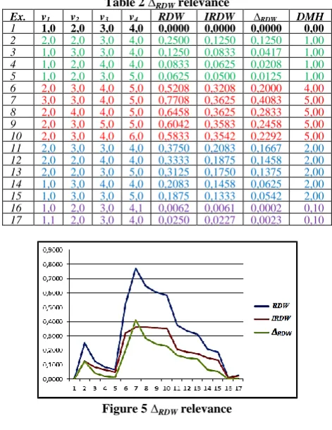
IRDW introduction was necessary to define another indicator that brings new advantages in dissimilarity measure using feature vectors. This new indicator, denoted by ΔRDW is the absolute value of difference between RDW and IRDW:
(8)
Experiments that reflect relevance ΔRDW are presented in Table 2.
Property6: ΔRDW indicator determine in Rn hyperspace a hyperplane HRDW with the property that all points in HRDW verify the relation ΔRDW = 0 in relation to the origin O = {0,0, ... 0) of Rn.
This means that zero values for ΔRDW and equal but nonzero values for RDW and IRDW for two or more feature-vectors does not mean that those vectors are identical, but they determine different points in a same hyperplane.
Property7: For the u and α constant and an uniform variation in the same direction (ascending or descending) with the same value ri (called ratio) of the feature-vectors vik, the function RDW(u, v, α) is linear and strictly monotone.
Property is not valid for RDWI(u,v,α) and for the ΔRDW(u,v,α). Property8: symmetry axiom.
Property9: RDW(u,v, α)=IRDW(v,u, α) and RDW(v,u, α)=IRDW(u,v, α)
The complexity of the problems to be solved often require hybrid feature-vectors, ie combinations of real and logical values. One such example would be the feature-vector of a matrix that can have features such as sparsity (real), symmetry (boolean), diagonally dominant (boolean), number of non-zero values (real) etc. The feature-vector splitting in two homogeneous vectors in terms of the data types and use an adequate measures for each -for example RDW for real values and DH (Hamming distance [1]) for logical values-, seems at first sight an acceptable solution. But after calculating separately these distances, the question is how do we classify accordingly if there are two indicators of different type. One option would be to convert the DH value from logical into a real value. This can be done with a good approximation if TRUE is replaced by 1 respectively FALSE with 0. Knowing that for two vectors u and v we have the Hamming distance
ie where
and using the substitutions
, will be obtained for DH(ui,vi) the values 1 or 0, which can be summed up to RDW value. An "adjustment" of these values regarding the boolean component contribution to the total value of RDW can be made using the appropriate component αi from the relevance vector α.
Therefore, the relation (6) becomes:
(9)
where
Important note: Generally, the feature-vectors values are strictly positive real numbers, or logical values and as a consequence there is no need of correction factor ɛ in relations
proposed before, which will increase accuracy and simplify the calculation.
3.
EXAMPLES AND COMMENTS
There were performed a series of experiments to study the relevance and properties of proposed indicator RDW and those derivates from it, IRDW and ΔRDW , resulting several observations as follows:
1) zero value for RDW(u,v,α) indicates a perfect similarity of the two vectors u and v (examples 1, 7, 13 and 19 in Table 1) and represents the ideal case for a classification problem;
2) the ideal case does not depend on relevance vector α
(examples 1,7,13 and 19 from Table 1;
3) experiments regarding the influence of feature-vector v:
[image:3.595.320.527.349.435.2]-for a uniform variation (with the same ratio) and strictly monotone of one or more components of vk on both sides of the reference vector u, is obtained linear and symmetrical variations of RDW values. RDW sequence values is unimodal and symmetric, as can be seen in Figure 2. This experiment exemplifies the theorem from the previous section. In example presented in figure 2 the working parameters was: u={1,2,3}, v=(v1,v2,v3}, , α={1,1,1}
Figure 2 An example for theorem: RDW(u,v,α) is unimodal
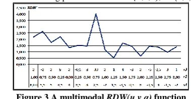
[image:3.595.326.516.497.596.2]-in Figure 3 is exemplified the case when at least for a feature in vk, the values sequence is not monotonous. In this case RDW(u,v,α) function is multimodal, with several minimum values. The working parameters was: u={1,2,3}, α={1,1,1};
Figure 3 A multimodal RDW(u,v,α) function
4) an example of property 3, ie RDW (u, v) ≠ RDW (v, u): if u = {1,2,3,4}, v={4,3,2,1} and α={1,1,1} is obtained RDW (u, v, α) = 1.203 and RDW (v, u, α) = 11.146;
5) examples for triangle inequality: if u={1,2,3,4}, a={2,4,6,8}, b={3,6,9,12} and α={1,1,1,1}, we obtain:
i)) RDW(u,a)=1, RDW(a,b)=0.5 and RDW(u,b)=2 ie RDW(u,b) > RDW(u,a) + RDW(a,b): not verify the triangle inequality;
but
6) The relevance-vector α affect only RDW values, without affecting the positions of minimum, global or local, on the abscissa, as can be seen in Figure 4.
Figure 4. The influence of relevance vector α
Also, it is possible to use different sequences for relevance-vector α depending on certain conditions, such as for example depending on vivalue. An example: for v1<10 will be used α={1,1,1} respectively α={2,1,1} for v1> = 10.
[image:4.595.76.264.107.207.2]7) The relevance of ∆RDWindicator can be seen in Table 2 respectively Figure 5. Working parameters was u={1,2,3,4} and α={1,1,1,1}. ΔRDW values close to zero show a greater degree of dissimilarity between vectors u and v.
Table 2 ∆RDWrelevance
Ex. v1 v2 v3 v4 RDW IRDW ∆RDW DMH
1 1,0 2,0 3,0 4,0 0,0000 0,0000 0,0000 0,00
2 2,0 2,0 3,0 4,0 0,2500 0,1250 0,1250 1,00
3 1,0 3,0 3,0 4,0 0,1250 0,0833 0,0417 1,00
4 1,0 2,0 4,0 4,0 0,0833 0,0625 0,0208 1,00
5 1,0 2,0 3,0 5,0 0,0625 0,0500 0,0125 1,00
6 2,0 3,0 4,0 5,0 0,5208 0,3208 0,2000 4,00
7 3,0 3,0 4,0 5,0 0,7708 0,3625 0,4083 5,00
8 2,0 4,0 4,0 5,0 0,6458 0,3625 0,2833 5,00
9 2,0 3,0 5,0 5,0 0,6042 0,3583 0,2458 5,00
10 2,0 3,0 4,0 6,0 0,5833 0,3542 0,2292 5,00
11 2,0 3,0 3,0 4,0 0,3750 0,2083 0,1667 2,00
12 2,0 2,0 4,0 4,0 0,3333 0,1875 0,1458 2,00
13 2,0 2,0 3,0 5,0 0,3125 0,1750 0,1375 2,00
14 1,0 3,0 4,0 4,0 0,2083 0,1458 0,0625 2,00
15 1,0 3,0 3,0 5,0 0,1875 0,1333 0,0542 2,00
16 1,0 2,0 3,0 4,1 0,0062 0,0061 0,0002 0,10
17 1,1 2,0 3,0 4,0 0,0250 0,0227 0,0023 0,10
Figure 5 ∆RDWrelevance
8) Comparison with other metrics
i) A set of experiments first were made under the conditions of theorem enunciated in section 2. An example can be seen in Figure 6.
Figure 6 Comparison with other metrics
[image:4.595.326.524.302.519.2]ii) There are situations when measures such as DMH, DE and DC, unlike RDW, have a low sensitivity, sometimes zero, to relative large variations in the features values of vi, which recommend the use of RDW measure in classification problems. An example of this is given in Table 3. Thus, for feature-vector values equal to {0,3,3}, {2,2,2} and {1,1,4} corresponding values for DMH, DE, DC+∞ and DC-∞ have the same values, while RDW values differs. In this example u = {1,2,3} and α = {1,1,1}.
Table 3 RDW relevance
v1 v2 v3 RDW DMH DE DC+∞ DC-∞
0 -1 -3 1,500 10 6,78 6 0
2 3 4 0,611 3 1,73 1 2
3 4 5 1,222 6 3,46 2 3
4 9 -2 2,722 15 9,11 7 4
4 8 -1 2,444 13 7,81 6 4
6 8 5 2,889 13 8,06 6 6
7 8 1 3,222 14 8,72 6 7
1 2 3 0,000 0 0,00 0 1
2 2 3 0,333 1 1,00 1 2
0 3 3 0,500 2 1,41 1 0
1 1 4 0,278 2 1,41 1 1
2 2 2 0,444 2 1,41 1 2
7 6 6 3,000 13 7,81 6 7
7 5 10 3,278 16 9,70 7 7
7 4 7 2,778 12 7,48 6 7
1 2 2 0,111 1 1,00 1 1
10 2 6 3,333 12 9,49 9 10
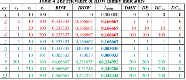
The advantage of using the ∆RDW in compared with other
indicators and way in which its values clearly indicate the extent to which vectors differ regardless of the size of the features is illustrated in Table 4. In this example, the three features have different orders of magnitude and example show very clearly the advantage of using ∆RDW to measure the
distance between two vectors, in the sense that it is not influenced by magnitude orders of features values.
Thus, in the first group (eg 2, 3 and 4) each feature value was doubled from baseline. In the three cases for the same variation in percent (100%) of each feature, it obtained the same variations for RDW, IRDW and ∆RDW, which is correct, unlike
the values obtained with other indicators.
[image:4.595.50.286.334.639.2]Table 4 The relevance of RDW family indicators
ex v1 v2 v3 RDW IRDW ∆RDW DMH DE DC+∞ DC+∞
1 1 10 100 0 0 0,000000 0 0 0 0
2 2 10 100 0,333333 0,166667 0,166667 1 1 1 0
3 1 20 100 0,333333 0,166667 0,166667 10 10 10 0
4 1 10 200 0,333333 0,166667 0,166667 100 100 100 0
5 2 10 100 0,333333 0,166667 0,166667 1 1 1 0
6 1 11 100 0,033333 0,030303 0,003030 1 1 1 0
7 1 10 101 0,003333 0,0033 0,000033 1 1 1 0
8 201 10 100 66,66667 0,331675 66,334992 200 200 200 0
9 1 210 100 6,666667 0,31746 6,349206 200 200 200 0
10 1 10 300 0,666667 0,222222 0,444444 200 200 200 0
4.
CONCLUSIONS
The definition and experiments show that RDW, IRDW and ∆RDW indicators are not influenced by orders of magnitude of
different features.
RDW, IRDW and ∆RDW are sensitive to percentual difference
in which is ui and vi are and not to the absolute difference between these values, as happens at DMH or DE indicators. The frequency of cases in which for very different feature-vectors are obtained equal values for RDW is much lower, even insignificant, in comparison with other indicators like DMH, DE or DC. Such situations -equal values for very different situations- can lead to wrong classifications. RDW values vary in a reasonable range of values, which is quite narrow, relatively independent of the orders of magnitude of the components from feature-vectors.
The RDW value is independent from the number of features, as happens for example to DMH and DE. This property allows in some cases to be excluded from the analysis an "uncomfortable" feature, without RDW value to be affected to a great extent.
Using the relevance vector α allows sensitization of RDW indicator to weight/importance of each feature in part. ΔRDW indicator, which is a measure of the difference between direct and inverse RDW distance bring added certainty regarding the degree of similarity of two feature-vectors, its low values indicating a "similarity "greater of those two vectors.
Values of characteristics from feature-vectors is most often the values of physical quantities, chemical, etc., often different, with different measurement units (pieces, m, m2, m3, kg, N, kg/m3 etc). The proposed approach is more natural in the sense that the value of RDW not having units of measurement (by simplification), its interpretation is simple and scientifically correct: "distance/difference between vector u and v is 7% compared to the reference-vector u ". In the case of other indicators may sound rather strange, "the distance between u and v is 16 kg-newtons-meters ...".
Through the substitutions true →1 and false → 0, RDW indicator can be used in situations where feature-vectors are hybrids (real and boolean values).
The immediate goal is to use the proposed indicator in a classification/recommendation system for partitioning systems of equations when solving these on a parallel computer. Twenty features of the associated matrix have been selected "size, bandwidth, average bandwidth [12], symmetry, positivity, sparsity, profile, euclidean norms, distributions of nonzero elements per row/column etc" for this purpose. Some of these features have been successfully used in the classification process, relevant examples are given by Shuting Xu in [13] and in his doctoral thesis [14] and by T. George in his doctoral thesis [15].
The first results, regarding partitioning in parallel conjugate gradient, are encouraging but inconclusive because we do not know yet what is the importance, the relevance and the weight of each feature in part on the mentioned parallel process. Studies and experiments in this direction will be made in the future.
Another future work is to use the proposed indicator in the selection/recommendation the preconditoning and the parallel numerical method for solving a system of linear equations.
5. REFERENCES
[1] R. Hamming, “Error detecting and error correcting codes”, The BellSystem Technical Journal, vol. XXVI, pp. 147–160, April 1950.
[2] Kruskal J.B., Multidimensional scaling by optimizing goodness of fit to a non metric hypothesis.” Psychometrika 29(1):1-2, 1964
[3] A. Bhattacharya, P. Kar, M. Pal, „On Low Distortion Embeddings of Statistical Distance Measures into Low Dimensional Spaces”, Springer, LNCS, Vol. 5690, pp 164-172, 2009
[4] K. Chaudhuri, A. McGregor, „Finding Metric Structure in Information-Theoretic Clustering”, in Proceedings of COLT 2008, pp. 391–402, 2008
[5] J.Yu, J. Amores, N. Sebe, Q. Tian, „A new study on distance metrics as similarity measurement”, IEEE Proc. ICME 2006, E ISBN:1-4244-0367-7, pp. 533 – 536, 2006
[6] J. Yu, J. Amores, N. Sebe, P. Radeva, Q. Tian ,”Distance Learning for Similarity Estimation”, IEEE Trans. on pattern analysis and machine intelligence, vol. 30, no. 3, march 2008
[7] A. Bookstein, S. T. Klein, T. Raita, „Fuzzy Hamming Distance: A New Dissimilarity Measure”, LNCS Vol. 2089, 2006, pp 86-97, Springer2006
[8] B.G. Park, K. M. Lee, S.U. Lee, „A New Similarity Measure for Random Signatures: Perceptually Modified Hausdorff Distance”, J. Blanc-Talon et al. (Eds.): ACIVS 2006, LNCS 4179, pp. 990–1001, 2006, Springer 2006
[9] M.P.Dubuisson, A.K.Jain, “A modified Hausdorff distance for object matching” Proc. of IEEE International Conference on Pattern Recognition,pp.566-568, October 1994.
IEEE Trans. Image Processing, vol.8, no.3, pp.425-428, March 1999.
[11] L. Wang, C. Yang, J. Feng, „On Learning with Dissimilarity Functions”, Proceedings of the 24th International Conference on Machine Learning, Corvallis, OR, 2007
[12] L.O. Mafteiu-Scai, V. Negru, D. Zaharie, O. Aritoni, Average bandwidth reduction in sparse matrices using hybrid heuristics, Studia Universitatis Babes-Bolyai University, Cluj Napoca, Volume LVI Number 3 Sept. 2011, pp 97-102, ISSN:1224-869x, 2011
[13] Shuting Xu, Jun Zhang, ”A new data mining approach to predict matrix condition number”, Communication in
information an systems 2004 International Press Vol.4, No.4, pp. 325-340, 2004
[14] Shuting Xu, "Study and Design of an Intelligent Preconditioner Recommendation System" (2005). Doctoral Dissertation Paper 327, University of Kentucky, http://uknowledge.uky. edu/gradschool_diss/327,2005
[15] T. George, „A Recommendation system for preconditioned iterative solvers”, Doctoral Dissert.
Texas A&M University,
http://repository.tamu.edu/bitstream/handle/1969.1/ETD-