Block Truncation Coding using Enhanced Interpolations and Lookup Procedures for Image Compression

Block Truncation Coding using Enhanced Interpolations

and Lookup Procedures for Image Compression

S.Vimala

Dept. of Comp. Sci. Mother Teresa Women’s

University Kodaikanal – 624 102

Tamil Nadu, India

P.Uma Edwin

Dept. of Comp. Sci. J.A.Arts and Sci. College

University of Madras Chennai, Tamilnadu, India

P.Anne Raja Reega

Ruth

Dept. Comp. Applications RVS College of Engineering and

Technology Dindigul – 624 005

Tamilnadu, India

ABSTRACT

Block Truncation Coding is one of the easy and efficient techniques for lossy image compression. In this paper, we have proposed few methods to enhance the existing Interpolative and Lookup procedures to reduce the bitrate and to improve the PSNR obtained with the Block Truncation Coding (BTC) based image compression methods. Of the existing BTC based methods, we have implemented the Minimum Mean Square Error (MMSE) method which gives better PSNR (quality of the reconstructed images) value to generate the bitplane and statistical moments. The size of the bitplane is reduced using Interpolation and Lookup procedures with noticeable degradation in PSNR value. This degradation is minimized using the proposed methods. Hence the proposed methods give less bitrate and better PSNR, when compared to the existing methods.

General Terms

Image Compression, Block Truncation Coding, Interpolative Techniques and Lookup Procedure.

Keywords

Image compression, bit-rate, bit-plane, BTC, PSNR, MMSE, Interpolation.

1.

INTRODUCTION

Generally image files occupy much storage and take more time for transmission. Images are being used in many areas like medical imaging, web applications, digital photos, satellite imaging, multimedia messaging in cellular phones etc. As the demand for images has become more now-a-days, an efficient image coding technique is essential. Image compression techniques [1] play a vital role in reducing the cost of storage and transmission.

Compression techniques deal with reducing the storage required to save the image and ultimately increase the transmission speed [2]. All types of images like binary, gray scale, color images, video frames can be compressed efficiently using various image compression techniques.

Image compression is of two types, lossy and lossless [3], [4]. For most applications, where little loss of data is not vital, lossy compression is used. Lossless techniques are suitable for medical imaging where a small loss in data may even lead to loss of human lives. Block Truncation Coding (BTC) [5], Vector quantization (VQ) [6], Discrete Cosine Transform (DCT) [7] and Discrete Wavelet Transformation (DWT) [8] are some of the lossy image compression methods. Of these techniques, BTC is a simple and fast image compression technique, introduced by Delp and Mitchell [5]. BTC is based on the conservation of statistical properties. Although it is a simple technique, BTC has plays an important role in the history of image compression. Many image compression techniques have been developed based on BTC [9]. It achieves 2 bits per pixel (bpp) with low computational complexity. It is easy to implement when compared to vector quantization [10] and transform coding [11], [12].

Some irrelevant data is removed when an image is compressed and hence the reconstructed image will not be exactly equal to the original image. The difference between the original image and the compressed image is called Mean Square Error (MSE) and is calculated using the equation (1).The quality of the reconstructed image called the Peak Signal to Noise Ratio (PSNR) is calculated using the equation (2) and is the inverse of MSE.

∑

=

−

=

N

i

i i

x

y

N

MSE

1

2

)

(

1

) (1)













=

MSE

PSNR

2 10

255

log

10

(2)

In this paper, we have incorporated our novel ideas in enhancing the existing Interpolation and Lookup procedures in MMSE (a BTC based method for image compression) to improve the performance in terms of bits per pixel (bpp) and PSNR.

In Section 2, we briefly outline the existing BTC, AMBTC, MMSE, New lookup and Interpolative methods. The proposed methods are explained in Section 3. The experimental results are discussed in Section 4 and the conclusion is given in Section 5.

2.

EXISTING

BTC

BASED

COMPRESSION TECHNIQUES

2.1

Standard Block Truncation Coding

In BTC method, the given image is divided into N number of non-overlapping blocks , each of size 4 x 4 pixels. For each

block, the statistical moments, the mean

x

and standard deviation σ are preserved and are calculated using the equations (3) and (4).

X

=

∑

= m

i

xi

m

1

1

(3)

σ

=

(

)

m

x

x

_i 2

∑

−

(4)

where xi represents the i th pixel value of the image block and m

is the total number of pixels in that block. Taking

x

as the threshold value, a two-level bit plane is obtained by comparing

each pixel value xi with the threshold value. If xi <

x

then the pixel is replaced with ‘0’, otherwise with ‘1’. By this process, each block is reduced to a bit plane of size 16 bits. The bit plane

along with

x

and σ form the compressed data. Hence a block of 4 x 4 pixels will give a 32 bit compressed data, amounting to 2 bpp [13]. To reconstruct the image at the receiving end, two quantizers a and b are computed using the equations (5) and (6). In the decoder, an image block is reconstructed by replacing 1’s in the bit plane with ‘b’ and the 0’s with ‘a’.

a

=

X

−

σ

m

q

q

−

(5)

b

=

X

+

σ

q

q

m

−

(6) where m-q and q are the number of 0’s and 1’s in the compressed bit plane respectively.

Please use a 9-point Times Roman font, or other Roman font with serifs, as close as possible in appearance to Times Roman

point text, as you see here. Please use sans-serif or non-proportional fonts only for special purposes, such as distinguishing source code text. If Times Roman is not available, try the font named Computer Modern Roman. On a Macintosh, use the font named Times. Right margins should be justified, not ragged.

2.2

Absolute Moment Block Truncation

Coding

Lema and Mitchell presented a simple and fast variant of BTC [14], named Absolute Moment BTC (AMBTC). In this method,

the higher mean

x

h _{and lower mean}

x

l _{are preserved instead}

of the mean and standard deviation values. Pixels in an image block are then classified into two groups of values. One group (higher range) comprising of gray levels which are greater than

or equal to the mean (

x

) and the remaining gray levels are

brought into another group (lower range). The mean

x

h of

higher range and

x

l _{of the lower range are calculated using the}

equations (7) and (8).

(

)

∑

<

−

=

x x

Xi l

i

q

m

x

1

(7)

∑

≥

=

x x

i h

i

x

q

x

1

(8) where q is the number of pixels whose gray levels are greater

than or equal to

x

. Then a two level quantization is performed for all the pixels in that block to form a bit plane of 1’s and 0’s.

For each block, the encoder generates

x

l _,

x

h _{and bitplane to}

a file thus leading to 2 bpp like BTC. But AMBTC involves less number of computations when compared to BTC as standard deviation involves more multiplications.

2.3. Minimum Mean Square Error (MMSE)

MMSE is the iterative process of AMBTC [15]. This technique is used to reduce the error (MSE value) between the original and the compressed images. In this method, the threshold value t is initialized by taking the average of minimum and maximum values of each block. The two statistical moments a and b are calculated using the equations (9) and (10) and are optimized as shown Fig. 1.

a = Xmin (9)

2.4.

BTC based on New Look-up Table

For the images with high correlation between adjacent pixels, the bit plane output which is binary in nature will also have a high degree of correlation between its adjacent bits. This feature is exploited to further reduce the size of bit-plane using the Interpolation and Lookup methods.

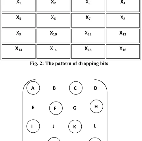
In new look-up table technique, consider the 4 x 4 bit-plane shown in Fig. 2. Because of high correlation among adjacent bits, the alternate bits, viz. the encircled ones alone are transmitted or stored. The dependent bits, viz. the bits other than encircled bits are dropped in the encoding stage and are interpolated from the values of the surrounding encircled bits [16] as shown in Fig. 3 in the decoding stage. This technique helps in reducing the size of bit-plane from 16 bits to just 8 bits.

Fig. 2: The pattern of dropping bits

A B

E

C D

F G H

I J K L

[image:3.612.66.276.68.416.2]

M N O P

Fig. 3: The bits to be retained are encircled

The interpolation is performed according to the following look-up table:

B = 1, iff two or more of the surrounding bits, viz. A, F, and C are equal to 1.

D = C

E = 1, iff two or more of the surrounding bits, viz. A, F, and I are equal to 1.

G = 1, iff two or more of the surrounding bits, viz. F, K, H and C are equal to 1.

J = 1, iff two or more of the surrounding bits, viz. F, K, N and I are equal to 1.

L = 1, iff two or more of the surrounding bits, viz. H, K and P are equal to 1.

M = N

O = 1, iff two or more of the surrounding bits, viz. N, K and P are equal to 1.

The corner bits, namely, D and M are set equal to C and N, respectively since the horizontal sampling process is likely to result in a high correlation in the horizontal direction than in the vertical direction. In Look-Up procedure, before mapping 1’s and 0’s to a and b respectively, the dropped bits are generated using the above conditions to generate a bit-plane of size 16 bits. This bit-plane is then transformed to approximate gray levels of original values.

X1 X2 X3 X4

X5 X6 X7 X8

X9 X10 X11 X12

X13 X14 X15 X16

a = xmin

b = xmax

t = (a+b)/2

(

−

)

∑

<

=

t x

Xi

i

q m

a' 1

∑

≥

=

t x

i

i

x q

b ' 1

is a’ == a & b’ == b

a & b are the output

levels

a = a’ & b = b’

[image:3.612.321.568.80.325.2]

2.5.

Interpolative Technique

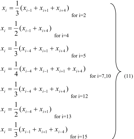
[image:4.612.55.283.335.572.2]

In this method, of the 16 components of the bit-plane, the boldfaced components as in Fig. 4 are dropped and hence the size of the bit-plane is 8 * 1 = 8 bits rather than 16 bits [13].

Fig. 4: Pattern of dropping bits in Interpolative Technique

In decoding phase, the dropped bits are recovered by taking the arithmetic mean of the adjacent pixel values as given in equations (11).

)

(

3

1

4 1

1 + +

−

+

+

=

_{i i i}

i

x

x

x

x

for i=2

)

(

2

1

4 1 + −

+

=

_{i i}

i

x

x

x

for i=4

)

(

3

1

4 1

4 + +

−

+

+

=

_{i i i}

i

x

x

x

x

for i=5

)

(

4

1

4 1 1

4 − + +

−

+

+

+

=

i i i i

i

x

x

x

x

x

for i=7,10 (11)

)

(

3

1

4 1

4 − +

−

+

+

=

_{i i i}

i

x

x

x

x

for i=12

)

(

2

1

1 4 + −

+

=

_{i i}

i

x

x

x

for i=13

)

(

3

1

4 1

1 + −

−

+

+

=

_{i i i}

i

x

x

x

x

for i=15

In interpolative method, the existing 8 bits are transformed into gray levels based on the quantizers. Once the approximate gray levels are generated, the gray values for the dropped bits are generated using the equations set (9).

3.

PROPOSED METHOD

In the proposed method, we have used MMSE technique for generating the bit-plane and the statistical moments High Mean and Lower Mean. The size of the bit-plane thus generated using

and henceforth the quality of the reconstructed images is significantly improved. As a result of the proposed scheme, there is improvement both in terms of bit-rate and the PSNR.

3.1. Modified Interpolative Method

In this method, the interpolative method is modified by means of assigning the nearest pixel with the top-left and bottom right corner pixels and remaining pixels are replaced with average of adjacent pixels. The dropped bits are shown in Figure 2. In encoding stage, the size of the bit plane is reduced to half of its original size. In decoding stage, Top-left and Bottom-right corner pixels are assigned the nearest pixel value and the remaining pixels are replaced with the mean of adjacent pixel values that are computed using the equations (12).

x_i = 1/3(x_i-1+x_i+1+x_i+4) for i = 2

xi = xi-1 for i = 4

xi = 1/3(xi-4+xi+1+xi+4) for i = 5

xi = 1/4(xi-4++xi-1+xi+1+xi+4) for i = 7, 10 (12)

xi = 1/3(xi-1+xi-4+xi+4) for i = 12

xi = xi+1 for i = 13

xi = 1/3(xi-1+xi+1+xi+4) or i = 15

3.2. Diagonal Interpolative Method

In this method, the diagonal pixels (boldfaced) are selected as permanent pixels and the remaining non diagonal pixels are replaced by taking the arithmetic mean of adjacent pixels. The dropping bits are shown in Figure 4. In decoding stage, the remaining pixels are computed using the equations (13).

)

(

2

1

4 1 + −

+

=

i i

i

x

x

x

for i = 2,12

)

(

2

1

4 1 + +

+

=

_{i i}

i

x

x

x

for i = 3,9

)

(

2

1

1 4 + −

+

=

_{i i}

i

x

x

x

for i = 5,15 (13)

)

(

2

1

4 1 − −

+

=

_{i i}

i

x

x

x

for i = 8,14

3.3. Non-Diagonal Interpolative Method

In this method, the Non-diagonal pixels (boldfaced) are selected as permanent pixels and the remaining diagonal pixels are replaced by taking the arithmetic mean of adjacent pixels. The bits to be dropped are shown in Fig. 5.

X1 X2 X3 X4

X5 X6 X7 X8

X9 X10 X11 X12

[image:5.612.46.290.67.185.2]

Figure 5 : The pattern of dropping bits in NDI Method.

In decoding stage, the remaining pixels are computed using the equations (14).

)

(

2

1

4

1 +

+

+

=

_{i i}

i

x

x

x

for i=1,11

)

(

2

1

4

1 +

−

+

=

_{i i}

i

x

x

x

for i=4,10 (14)

)

(

2

1

4

1 −

−

+

=

_{i i}

i

x

x

x

for i=6,16

)

(

2

1

4

1 −

+

+

=

_{i i}

i

x

x

x

for i=7,13

3.4. Diagonal Look-Up (DL) Method

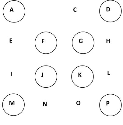
[image:5.612.333.535.277.479.2]

In this method, the bit plane is reduced to half of its size by dropping the diagonal bits in the bit plane. In Fig. 6, circled bits are selected and the remaining bits are dropped.

Fig. 6: The pattern of dropping bits in DL Method

In decoding stage, the dropped bits are regenerated as follows:

B = 1 or E = 1 iff one or more of the surrounding bits, viz. A and F are equal to 1.

C = 1 or H = 1 iff one or more of the surrounding bits, viz. D and G are equal to 1.

I = 1 or N = 1 iff one or more of the surrounding bits, viz. M and J are equal to 1.

L = 1 or O = 1 iff one or more of the surrounding bits, viz. K and P are equal to 1.

3.4. Non-Diagonal look-Up Method

In this method, the bit plane is reduced to half the size by dropping the non-diagonal bits in the bit plane. In Fig. 7, the circled bits are selected and the remaining bits are dropped.

Fig. 7: The pattern of dropping bits in NDL method

In decoding stage, the remaining bits are assigned as follows:

A = 1 iff one or more of the surrounding bits, viz. B and E is equal to 1

D = 1 iff one or more of the surrounding bits, viz. C and H is equal to 1

M = 1 iff one or more of the surrounding bits, viz. I and N is equal to 1

P = 1 iff one or more of the surrounding bits, viz. L and O is equal to 1

F = 1 iff two or more of the surrounding bits, viz. A, B and E is equal to 1

G = 1 iff two or more of the surrounding bits, viz. C, D and H is equal to 1

J = 1 iff two or more of the surrounding bits, viz. I, M and N is equal to 1

K = 1 iff two or more of the surrounding bits, viz. L, P and O is equal to 1

X1 X2 X3 X₄

X5 X6 X7 X8

X9 X10 X11 X12

X13 X14 X15 X16

D

C

A

K

E

I

F

L

H

N

O

P

G

J

M

D

C

A

B

K

E

I

F

L

H

N

O

P

G

J

[image:5.612.70.272.434.640.2]

4.

RESULTS AND DISCUSSION

Experiments were carried out with standard images Cameraman, Boats, Bridge, Baboon, Lena and Kush of size 256 x 256 pixels. The input images taken for the study are given in Fig. 8.

(a) Cameraman (b) Boats

(c) Bridge (d) Baboon

[image:6.612.337.537.78.201.2]

(e) Lena (f) Kush

Fig. 8: Input Images taken for the Study

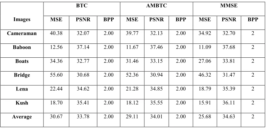
The algorithm is implemented using MATLAB 7.0 on Windows operating system. The hardware used is the Intel® 3.06GHz Processor with 512 MB RAM. The different methods of BTC are implemented and the results are displayed in tables. The PSNR value is taken as a measure of the quality of the reconstructed image. The MSE, PSNR and the bpp values that are obtained with the BTC, AMBTC and MMSE (existing BTC based techniques) for six different standard test images are presented in Table 1.

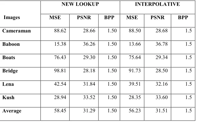
Table 2: The MSE, PSNR and BPP values for New Lookup and Interpolative Methods

Images

NEW LOOKUP INTERPOLATIVE MSE PSNR BPP MSE PSNR BPP Cameraman 88.62 28.66 1.50 88.50 28.68 1.5

Baboon 15.38 36.26 1.50 13.66 36.78 1.5

Boats 76.43 29.30 1.50 75.64 29.34 1.5

Bridge 98.81 28.18 1.50 91.73 28.50 1.5

Lena 42.54 31.84 1.50 39.51 32.16 1.5

Kush 28.94 33.52 1.50 28.35 33.60 1.5

[image:6.612.152.482.436.641.2]

[image:7.612.95.525.173.381.2]

The BTC, AMBTC and MMSE methods are used to generate the bit-plane and the statistical moments for each block of the input image. The size of the bit-plane thus generated by any of the aforementioned methods is further reduced using any one of the existing Interpolative or New Lookup methods. The Interpolative and New Lookup methods are used to reduce the size of the bit-plane to half of its original size.

Table 2. gives the results obtained with the MMSE method New Lookup and Interpolative methods in terms of MSE, PSNR and BPP. It is observed that there is no much difference between the results of both the techniques. Using Interpolative and New Lookup procedures, the bit-rate has been reduced from 2 bpp to 1.5 bpp.

Table 1: The MSE, PSNR and BPP values of Existing BTC methods

Images

BTC AMBTC MMSE

MSE PSNR BPP MSE PSNR BPP MSE PSNR BPP Cameraman 40.38 32.07 2.00 39.77 32.13 2.00 34.92 32.70 2

Baboon 12.56 37.14 2.00 11.67 37.46 2.00 11.09 37.68 2

Boats 34.36 32.77 2.00 31.46 33.15 2.00 27.06 33.81 2

Bridge 55.60 30.68 2.00 52.36 30.94 2.00 46.32 31.47 2

Lena 22.44 34.62 2.00 21.28 34.85 2.00 18.79 35.39 2

Kush 18.70 35.41 2.00 18.12 35.55 2.00 15.91 36.11 2

Average 30.67 33.78 2.00 29.11 34.01 2.00 25.68 34.63 2

[image:7.612.140.479.481.733.2]

Table 3. gives the results of Proposed Methods (Enhanced Interpolative (EI), Diagonal Interpolative (DI), Non-Diagonal Interpolative (NDI), Diagonal Lookup (DL) and Non-Diagonal Lookup (NDL)) in terms of MSE, PSNR and BPP. As the size of the bit-plane is reduced, the bpp has been reduced from 2 to 1.5, which is a significant improvement in bit-rate.

Table 3: MSE, PSNR and BPP values obtained with the proposed method Method Cameraman Baboon Boats Bridge Lena Kush Average

EI

PSNR 29.52 37.29 30.69 28.90 33.31 34.37 32.35

BPP 1.5 1.5 1.5 1.5 1.5 1.5 1.5

DI

PSNR 28.64 36.12 29.78 28.23 32.50 33.55 31.47

BPP 1.5 1.5 1.5 1.5 1.5 1.5 1.5

NDI

PSNR 28.91 36.63 29.82 28.34 32.63 33.79 31.69

BPP 1.5 1.5 1.5 1.5 1.5 1.5 1.5

DL

PSNR 30.71 37.31 32.85 30.26 34.19 35.18 33.42

BPP 1.5 1.5 1.5 1.5 1.5 1.5 1.5

NDL

PSNR 31.24 37.78 32.91 30.35 34.42 35.53 33.71

But the PSNR has been reduced from 34.63 to 31.51. The proposed methods give better PSNR when compared to that of existing interpolation and lookup methods. The PSNR values obtained with the proposed Interpolative and Lookup methods are given in Table 3. The PSNR has been raised from 31.51 to 33.71. This is a significant improvement.

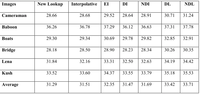
Table 4 gives the PSNR values obtained with the existing Interpolative and New Lookup procedures and the proposed methods. The average PSNR obtained with the existing Interpolative and New Lookup methods are 31.29 and 31.51 respectively. The bpp of both the methods is 1.5. With the proposed ideas incorporated in the existing methods, the PSNR is raised to an average of 33.71 with a bpp of 1.5. The average PSNR obtained with the BTC, AMBTC and MMSE techniques are 33.78, 34.01 and 34.63 respectively with a bpp of 2. But the proposed methods the reduce the bpp from 2 to 1.5 only with the slight reduction in PSNR. When compared to normal BTC, the bpp is reduced to 1.5 from 2 bpp only with a negligible loss in PSNR, i.e. only 0.07. The PSNR obtained with the existing Lookup method has been raised to 33.71 from 31.51, which is a significant improvement.

When the MMSE method is implemented with New Lookup and Interpolative techniques, the average bpp has been reduced from 2 bits to 1.5. bpp, which is a significant reduction in bpp. But the PSNR has been reduced from 34.63 to 31.51. This is a noticeable degradation. This degradation is reduced with the proposed interpolation methods and the PSNR has improved from 31.51 to 33.71 without affecting the bpp. Various orders of interpolation have been tried and the results obtained with the Non Diagonal Look-up (NDL) are good when compared with

5. CONCLUSION

Various orders of interpolation and lookup procedures for reducing the size of the bitplane in BTC based image compression methods are discussed in this paper. The experiments are conducted with standard gray scale images and the performance of all methods is measured in terms of PSNR and bpp. The existing interpolation and lookup methods reduce the bitrate from 2 bpp to 1.5 bpp with noticeable degradation in PSNR. On an average, the PSNR obtained with the existing methods is 31.51. But the proposed methods, when implemented with MMSE method, give better PSNR values. Of all the proposed methods, the Non Diagonal Lookup (NDL) method gives better results in terms of PSNR. The average PSNR obtained for all images is 33.71, which is a significant improvement. As the gray scale images form the base for color images, the NDL method can also be used for color images. These techniques are best suitable for imaging applications in hand-held devices.

6. REFERENCES

[1] K.Somasundaram and P.A.Kalaividya, “Design of Small Codebook for Vector Quantization Method for Still Image Compression”, Image Processing, NCIMP, Allied Publishers, 2010.

[2] Rafael C. Gonzalez, Ritchard E. Woods, “Digital Image Processing”,Pearson, 3rd Edition

[3] IM. Pu, Fundamental Data Compression, Oxford, Great Britan, Butterworth–Heinemann, 2006.

[image:8.612.127.514.127.310.2]

[4] David Salomon, Data Compression the Complete In Table 4, the PSNR values obtained with the proposed interpolative and lookup methods are compared with that of the existing interpolative and lookup methods.

Table 4. PSNR values of existing methods and the proposed methods

Images New Lookup Interpolative EI DI NDI DL NDL Cameraman 28.66 28.68 29.52 28.64 28.91 30.71 31.24

Baboon 36.26 36.78 37.29 36.12 36.63 37.31 37.78

Boats 29.30 29.34 30.69 29.78 29.82 32.85 32.91

Bridge 28.18 28.50 28.90 28.23 28.34 30.26 30.35

Lena 31.84 32.16 33.31 32.50 32.63 34.19 34.42

Kush 33.52 33.60 34.37 33.55 33.79 35.18 35.53

[5] E.J. Depp and O.R. Mitchell, “Image Compression using Block Truncation Coding”, IEEE Transactions on Communications, Vol. 27, pp. 1335–1342, 1979. [6] Y.Linde, A. Buzo, and R.M. Gray, An Algorithm for

vector quantizer design”, IEEE Transaction on Communications,Vol. COM-28, pp. 84–95, 1980. [7] G. K. Wallace, “Overview of the JPEG (ISQ/CCITT)

still image compression”, Proc. SPIE, Vol. 1244, pp. 220–233, 1990.

[8] A.Abbate, C.M. DeCusatis and P.K. Das, Wavelets and Subbands, Fundamentals and Applications, Boston, USA, Birkhauser, 2002.

[9] P.Franti, O.Nevalainen and T.Kaukoranta, “Compression of digital images by block truncation coding: a survey.”, The computer Journal, Vol. 37 issue 4, pp 308-332, 1994

[10] N.M.Nasrabadi, R.B. King, Image coding using vector quantization: a review, IEEE Transactions on Communications COM-36, pp. 957-971, 1998

[11] B.Pennebaker, and J.L.Mitchell, JPEG Still Image Data compression Standard., New York, Van Nosttrand Reinhold,1993.

[12] M. Rabbani and R. Joshi, ‘‘An overview of the JPEG 2000 still image compression standard,’’ Signal Process. Image Commun. Vol. 17, pp. 3–48, 2002.

[13] K.Somasundaram and I.Kaspar Raj, “Low Computational Image Compression Scheme based on Absolute Moment Block Truncation Coding”, World Academy of Science, Engineering and Technology, pp. 166-171, 2006

[14] Maximo D.Lema, O.Robert Mitchell, ”Absolute Moment Block Truncation Coding and its Application to Color Images”, IEEE Transactions on Communications, VOL. COM-32, NO. 10, October 1984

[15] Lucas Hui, “An Adaptive Block Truncation Coding Algorithm for Image Compression”, IEEE, PP.2233-2235, 1990.