Munich Personal RePEc Archive
Does monetary policy have differential
state-level effects? an empirical
evaluation
Nachane, D M and Ray, P and Ghosh, S
23 November 2001
Online at
https://mpra.ub.uni-muenchen.de/2708/
Does Monetary Policy Have Differential
State-Level Effects?
An Empirical Evaluation
The paper examines whether monetary policy has similar effects across major states in the
Indian polity. Impulse response functions from an estimated Structural Vector Auto
Regression (SVAR) reveal two sets of states: a core of states that respond to monetary
policy in a significant fashion vis-à-vis others whose response is less significant. The paper
attempts to trace the reasons for the differential response of these two sets of states in terms
of financial deepening and differential industry mix.
policies pursued). In the Indian context, although there have been several studies as to the impact of monetary policy on the national economy, there has been little investigation of the interrelationships among sub-national economies and asso-ciated feedbacks from policy shocks.1
Con-sequently, no comprehensive look at state-level response to a policy change is avail-able. Also lacking is a systematic analysis of why state economies may respond dif-ferently to monetary policy shocks. This is surprising, since state-level data offer a rich avenue for exploring the empirical significance of possible transmission mechanisms for monetary policy. The present paper attempts to address this lacuna by presenting a state-level analysis of monetary policy effects. Rather than con-fining itself to merely identifying dif-ferential responses, it also seeks to inves-tigate the reasons for such differential re-sponses. We follow the SVAR methodo-logy that claims as a major advantage its ability to identify monetary policy shocks adjusted for the influences of other concurrent developments.
Our analysis reveals that the response of different states to monetary policy shocks is, in fact, quite distinct. The size of a state’s response to a monetary policy shock is positively related to the share of manu-facturing in the NSDP (net state domestic product), which may be viewed as evi-dence favouring an ‘interest rate channel’. The analysis also provides support for the fact that certain states, containing a rela-tively larger concentration of small firms, tend to be more responsive to monetary policy shocks than states with a smaller concentration of the same, which, in
essence, is testimony to the existence of a ‘broad credit channel’.
II
Differential Impact of
Monetary Policy:
Issues and Empirics
The literature on the monetary transmis-sion mechanism suggests several reasons why the actions of the authorities might have differential state-level effects. These include, among others (i) statewise differ-ences in the mix of interest sensitive in-dustries, (ii) differences in the mixture of large versus small firms across states, and (iii) the differential financial deepening across states.
Differential Industry Mix
It is, acknowledged that the interest rate elasticities of credit demand differ across industries. These differential elasticities, in conjunction with differing industry mixes across states, may account for differential sub-national effects of mone-tary policy. It is also a stylised fact that industry is more credit-dependent than either agriculture or services and there-fore, relatively industrialised states are likely to be more affected by monetary policy shocks than their less industrialised counterparts.
Differential Mix of Firms
State-level differences in the composi-tion and concentracomposi-tion of industry and the sources of credit available to each could also lead to dissimilar responses to
I
Introduction
T
he prevailing paradigm of monetary policy predicates a uniform un-differentiated effect of such policy on the national economy. Such a view ignores the fact that in reality, any nation is composed of diverse albeit interlinked regions, which might respond differently to identical macroeconomic stimuli. For example, the effect of a change in the price of foodgrains might be quite different for a region which is a dominant producer of that commodity vis-à-vis another region, which is an important consumer. Likewise, a rise in the energy price (for example, fuel) might impact different regions un-evenly, in view of the differential impor-tance of fuel in the consumption basket of various regions. The idea that monetary policy can likewise have varied effects across regions is a short and logical next step.In large federal structures like the US, Canada and India, an additional dimension is introduced by the existence of compo-nent federal states with their own govern-ments and a measure of policy autonomy. While the concept of an economic region is logically quite distinct from that of a federal state, the latter provides a conve-nient anchor for studying regional dimen-sions of macroeconomic policy. This is so because in most countries, data is organised statewise rather than according to eco-nomic regions and also over a historical period, states develop distinct economic characteristics (partly due to inherent geographical and environmental features and partly owing to differing economic
monetary policy. The credit view of monetary policy, enunciated by Bernanke and Blinder (1988), contends that mon-etary policy affects banks by directly af-fecting their ability to provide loans. Moreover, information costs and transac-tions costs require small firms to deal with financial intermediaries, primarily banks, to meet their credit needs. In contrast, large firms usually have greater and varied access to external, non-bank sources of funds. Consequently, activity in a state that has a high concentration of small firms could be especially sensitive to the policy of the monetary authorities.
Differential Financial Deepening
Recent theoretical work on possible credit channels for the transmission of monetary policy actions to economic ac-tivity suggests that the mix of large versus small firms and large versus small banks is a crucial determinant of responses to monetary policy. Kashyap and Stein (1997) have pointed out that monetary policy is likely to have a relatively larger impact on countries having comparatively bank-de-pendent firms and a relatively large per-centage of small banks. The credit channel will be weakest in countries with a rela-tively low percentage of small banks and comparatively few bank-dependent cus-tomers. Dornbusch et al (1998) observe that, with the exception of the UK, the credit channel is more likely to be impor-tant in Europe, where banks provide the bulk of firms’ credit. In contrast, financing in the US (and in the UK) is much less bank-centric because capital markets play a central role in the financing of firms. In the Indian context, the process of financial deepening has not been uniform across states. Some states have experienced a significant growth of banking and insur-ance activities vis-a-vis certain other states which have remained relatively under-banked. It might therefore be possible to envisage a situation wherein adequately banked states are more prone to the effects of a monetary policy shock as compared with those which are not.
Differential Regional Impact of Monetary Policy: The Empirics
Some of the earlier literature in this area had investigated the effects of monetary policy on inter-regional banking flows, as opposed to economic activity. In one of the earliest regional studies for the US,
Miller (1978) found that Fed policy actions do not affect regional banking flows dif-ferently. Typical of these studies is the use of a reduced form equation that regresses personal income, earning or employment on the federal government revenues and the national money supply. These models are applied at the regional level to test the proposition that monetary policy has an important impact on nominal income. An important study in this context is Garrison and Chang (1979), which examines the effect of monetary policy on income vari-ables in the eight regions2 of the US. Their
study finds that monetary policy has dif-ferential effects across regions, with an especially large impact in the Rocky Mountain region. In contrast, Garrison and Kort (1983) investigate the impact of
monetary policy on state-level employ-ment for the 1960-78 period and find that states comprising the Great Lakes region are relatively more responsive to money supply changes, while states in the Rocky Mountain were the least responsive to such changes.
[image:3.567.211.535.274.681.2]A major shortcoming of such studies is their attempt to measure monetary policy impact region-by-region, without account-ing for feedback effects among regions. More recently, Taylor and Yucel (1996) have attempted to rectify this drawback by using a VAR to incorporate the inter-regional linkages, but their study is con-fined to a small time period (1982-95) and considers only four states, which, in a way, limits the empirical appeal of the model. Subsequently, Carlino and Defina (1998,
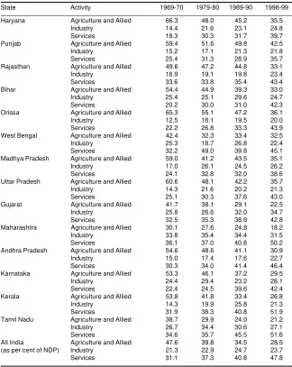
Table 1: Structure of NSDP in Different States
(as per cent of statewise NSDP)
State Activity 1969-70 1979-80 1989-90 1998-99
Haryana Agriculture and Allied 66.3 48.0 45.2 35.5
Industry 14.4 21.6 23.1 24.8
Services 19.3 30.3 31.7 39.7
Punjab Agriculture and Allied 59.4 51.6 49.8 42.5
Industry 15.2 17.1 21.3 21.8
Services 25.4 31.3 28.9 35.7
Rajasthan Agriculture and Allied 49.6 47.2 44.8 33.1
Industry 16.9 19.1 19.8 23.4
Services 33.6 33.8 35.4 43.4
Bihar Agriculture and Allied 54.4 44.9 39.3 33.0
Industry 25.4 25.1 29.6 24.7
Services 20.2 30.0 31.0 42.3
Orissa Agriculture and Allied 65.3 55.1 47.2 36.1
Industry 12.5 18.1 19.5 20.0
Services 22.2 26.8 33.3 43.9
West Bengal Agriculture and Allied 42.4 32.3 33.4 32.5
Industry 25.3 18.7 26.8 22.4
Services 32.2 49.0 39.8 45.1
Madhya Pradesh Agriculture and Allied 59.0 41.2 43.5 35.1
Industry 17.0 26.1 24.5 26.2
Services 24.1 32.8 32.0 38.6
Uttar Pradesh Agriculture and Allied 60.6 48.1 42.2 35.7
Industry 14.3 21.6 20.2 21.3
Services 25.1 30.3 37.6 43.0
Gujarat Agriculture and Allied 41.7 38.1 29.1 22.5
Industry 25.8 26.6 32.0 34.7
Services 32.5 35.3 38.9 42.8
Maharashtra Agriculture and Allied 30.1 27.6 24.8 18.2
Industry 33.8 35.4 34.4 31.5
Services 36.1 37.0 40.8 50.2
Andhra Pradesh Agriculture and Allied 54.6 48.6 41.1 30.9
Industry 15.0 17.4 17.6 22.7
Services 30.3 34.0 41.4 46.4
Karnataka Agriculture and Allied 53.3 46.1 37.2 29.5
Industry 24.4 29.4 23.2 28.1
Services 22.4 24.5 39.6 42.4
Kerala Agriculture and Allied 53.8 41.8 33.4 26.8
Industry 14.3 19.9 25.8 21.3
Services 31.9 38.3 40.8 51.9
Tamil Nadu Agriculture and Allied 38.7 29.9 24.0 21.2
Industry 26.7 34.4 30.6 27.1
Services 34.6 35.7 45.5 51.6
All India Agriculture and Allied 47.6 39.8 34.5 28.5 (as per cent of NDP) Industry 21.3 22.9 24.7 23.7
Services 31.1 37.3 40.8 47.8
1999) have attempted to rectify this short-coming by examining how monetary policy affects real personal income in each of the 48 contiguous states of the US. The analysis employs SVAR models estimated over the period 1958:1 to 1992:4; these models explicitly allowed for feedback among regions. Impulse response func-tions from the estimated SVARs revealed a broad pattern in which state real personal income tended to fall after an unantici-pated increase of one percentage point in the federal funds rate. Nonetheless, the differences in state responses are evident, and in some cases, substantial.
In the European context, Ramaswamy and Sloek (1997) found that the full effect of an unanticipated contraction in mone-tary policy on output in Austria, Belgium, Finland, Germany, Netherlands and UK takes roughly twice as long to occur and is twice as deep as in Denmark, France, Italy, Portugal, Spain and Sweden. Using VAR techniques, Gerlach and Smets (1996) found that while the effects of monetary policy shocks were not vastly different across countries in their study, they were somewhat larger in Germany than in France or Italy. Dornbusch et al (1998) have also employed a small model of six European countries and found that the impact effect of a monetary policy shock (changes in short-term interest rates) has a lag of eight months in Italy, Spain, Sweden and UK, nine months in Germany and 12 months in France. In sum, while these studies tend to disagree on an individual country’s responsiveness to monetary policy shocks, they are broadly in consonance with the fact that sensitivity to these shocks will differ across European countries.
Similar problems have come to the fore in the context of the European Monetary Union (EMU). Under the EMU, member countries will be subject to common monetary policy shocks. Given the diver-sity in the economic and financial struc-tures across the EMU economies, these common monetary shocks can be reason-ably expected to have differential effects. However, little is known about what dif-ferences might arise, given the absence of any historical experience in Europe with a common currency. In a pioneering study, Bayoumi and Eichengreen (1992), using a SVAR approach, demonstrated that the incidence of supply disturbances was very different for countries at the centre of the European community (the ‘core’ coun-tries) comprising of Germany, France, Belgium, Netherlands and Denmark)
vis-a-vis the other EC members (UK, Italy, Spain, Portugal and Greece). In particular, supply shocks to the ‘core’ countries were both smaller and more correlated across neighbouring countries as compared with supply shocks to the ‘non-core’ (or peri-phery) countries. This would seem to suggest that a uniform monetary policy might not necessarily produce the desired results under an EMU.
Some Indian Issues
The majority of the regional studies in the Indian situation have focused on examining the issue of state finances [Venkataraman 1967; Bagchi et al 1992], widening interstate disparities [Kurian 2000], their macroeconomic performance and differential interstate inequalities [Ahluwalia 2000], and sources of differ-ences in per capita state domestic product [Dasgupta et al 2000], variations in size, in-come and structural characteristics of states [Shand and Bhide 2000], and dispersion
of per capita incomes of states vis-à-vis the national average [Chaudhuri 2000]. The Reserve Bank of India has also been bring-ing out the status of state finances annually since 1950. Since the nation comprises of several states with not only differential growth patterns [Ahluwalia 2000] but also differential abilities to respond to mone-tary policy shocks, it would be of interest to understand the extent of such reactions at the state-level and this aspect is the predominant concern of our study.
III
Some Stylised Facts
on Indian States
[image:4.567.197.525.339.480.2]We have confined our attention to 14 major Indian states, viz, Haryana, Punjab, Rajasthan, Bihar, Orissa, West Bengal (WB), Madhya Pradesh (MP), Uttar Pradesh (UP), Gujarat, Maharashtra, Andhra Pradesh (AP), Karnataka, Kerala, and Tamil Nadu. However, the sample contains all the major states of India and
Table 2: Share of Unregistered Manufacturing in NSDP in Different States
(as per cent of statewise NSDP)
State/Year 1969-70 1979-80 1989-90 1998-99
Haryana 3.2 4.0 7.7 6.6
Punjab 4.0 5.4 6.6 5.2
Rajasthan 6.7 5.3 5.1 4.8
Bihar 14.1 3.2 7.1 1.9
Orissa 2.8 3.3 4.4 4.8
WB 4.5 3.5 8.4 8.6
MP 4.5 5.1 5.6 6.6
UP 4.7 6.7 5.6 5.5
Gujarat 4.4 4.2 6.0 9.2
Maharashtra 5.9 5.7 7.4 8.7
Andhra Pradesh 5.6 5.2 4.1 5.6
Karnataka 7.7 9.5 4.3 9.7
Kerala 3.8 6.9 5.6 6.5
Tamil Nadu NA 11.8 7.1 7.8
All India (as per cent of NDP) 5.4 6.0 5.9 5.7
Source: Central Statistical Organisation and Directorates of Economics and Statistics of respective state governments.
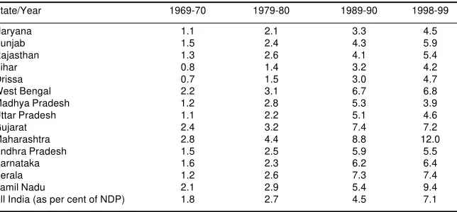
Table 3: Share of Banking and Insurance in NSDP in Different States
(as per cent of statewise NSDP)
State/Year 1969-70 1979-80 1989-90 1998-99
Haryana 1.1 2.1 3.3 4.5
Punjab 1.5 2.4 4.3 5.9
Rajasthan 1.3 2.6 4.1 5.4
Bihar 0.8 1.4 3.2 4.2
Orissa 0.7 1.5 3.0 4.7
West Bengal 2.2 3.1 6.7 6.8
Madhya Pradesh 1.2 2.8 5.3 3.9
Uttar Pradesh 1.1 2.2 5.1 4.6
Gujarat 2.4 3.2 7.4 7.2
Maharashtra 2.8 4.4 8.8 12.0
Andhra Pradesh 1.5 2.5 5.9 5.5
Karnataka 1.6 2.3 6.2 6.4
Kerala 1.2 2.6 7.3 7.4
Tamil Nadu 2.1 2.9 5.4 9.4
All India (as per cent of NDP) 1.8 2.7 4.5 7.1
[image:4.567.202.524.531.681.2]it is also in line with the standard practice in comparing the economic performance of Indian states that treats smaller or north-eastern states differently.3 The sample
period for the study is the 30-year period 1969-70 through 1988-99. As our interest is primarily on regional impact of mon-etary policy, we did not consider the pre-1970s (that is, pre-bank nationalisation) in our sample period.
How far do these states differ structur-ally? Table 1 provides an overview of the structure of net state domestic product (NSDP) at four representative time points encompassing the time period under study (1969-1999). As is evident from the table, at the all-India level, while the degree of industrialisation has increased over the period, certain states have witnessed a greater degree of industrialisation vis-à-vis the all-India average. Illustratively, during 1969-70, while the industrialisation at the all-India level as per cent of NDP was 21.3 per cent, the same for Orissa was merely 12.5 per cent as compared to Maharashtra at 33.8 per cent. Although the extent of industrialisation went up during 1989-90 to 24.7 per cent at the all-India level, states like Rajasthan and Orissa continued to lag behind their more developed counterparts like Maharashtra and Gujarat.
This apart, various states have differing degree of formalism in their economic activity. As regards the role of industry mix, Table 2 shows the share of unregis-tered manufacturing in NSDP in the con-cerned states at the four benchmark time points mentioned above. Without loss of generality, unregistered manufacturing would indicate the dominance of small units in a particular state. As compared with the all-India average of 5.5-6.0 per cent over the entire time span covered, certain states have a relatively high pro-portion of such firms. Notable among these include Haryana and West Bengal (espe-cially in the latter half of the 1980s and the 1990s); among others, Maharashtra and Tamil Nadu have had a significant proportion of unregistered manufacturing in NSDP, although for the latter, the pro-portion has declined in the latter half of the eighties. The same for Karnataka has also remained at a high level, albeit with a significant fall in 1989-90.
The evidence is corroborated when we consider the penetration of banking and insurance in the sample states (Table 3). States like Maharashtra, Gujarat, and to a lesser extent, Kerala, Tamil Nadu and West Bengal have a significant presence in
banking and insurance as evidenced from the share of these sectors in NSDP vis-à-vis the all-India average. For in-stance, during 1998-99, while the share of banking and insurance in NSDP for Maharashtra was 12.0 per cent, the same for Gujarat, Kerala and Tamil Nadu was 7.2, 7.4 and 9.4 per cent, respectively. As compared to this, the penetration of banking and insurance in states like Rajasthan, Bihar, Madhya Pradesh and Uttar Pradesh witnessed a declining trend over the period.
IV
Empirical Exploration:
Methodology and Results
The available literature tends to suggest several possible channels through which monetary policy could impinge differen-tially across regions. These include, for instance, state-level differences in the mix of industries, in the number of small versus large firms and in the extent of financial deepening.
In order to test our hypothesis that whether monetary policy shocks have differential effects in different states in India, we employ a vector auto regression (VAR) framework, with state-specific SDP, economywide GDP, monetary policy, and a variable capturing struc-tural shock. Towards this end, the study employs annual data on NSDP for the 14 major states in India as mentioned earlier for the period 1969 to 1999 for which consistent data set is available.4 In
addi-tion, we also have the real gross domestic product at the national level, an index of food price and an indicator of monetary policy shock, viz, the growth rate of real money supply, defined as (M3/P).5 The
inclusion of Pf/P in the VAR deserves
some explanation. Emerging market econo-mies are often susceptible to shocks in food prices. Food, in particular, consti-tutes a dominant proportion of their con-sumption basket and especially so in rela-tively backward states, where a significant part of incomes is often spent on food. Keeping this in mind, an index of food prices has been included as an additional variable.
The Framework
The analysis focuses on the dynamic behaviour of an n x 1 co-variance station-ary vector defined by the relation
Zt = [Yti, Y
t, (M3/P)t, (Pf/P)t]' (1)
where, Y is the NDP, Yi is the NSDP in
state i, Pf/P is an index of food price and M3/P is the monetary policy variable.
t denotes time period.
The dynamics of Zt are represented by
a VAR
AZt = B(L)Zt–1 + et (2) where A is an n x n matrix of coefficients describing the contemporaneous correla-tion among the variables, B(L) is an n x n matrix of polynomials in the lag operator L, and et = [ε1,t, ε2,t, …, εn–1,t, εn,t] is an n x 1 vector of structural distur-bances.
Solving for Zt produces the following
reduced form system
Zt = C(L)Zt–1 + ut (3) where, C(L) =A–1B(L) is an infinite-order
lag polynomial, and ut = A–1et describes
the relationship between the model’s reduced-form residuals and the model’s structural residuals.
[image:5.567.381.538.496.664.2]In order to achieve exact identification, instead of using Sims (1980) type trian-gular decomposition, sufficient restrictions are placed on the variance-covariance matrix of structural errors. For an exact identification, six restrictions have been placed on the A matrix. These are motiva-ted by practical consideration of the trans-mission of economic changes through sub-national and sub-national economies. In parti-cular, we have assumed that the food price shock is unrelated to other shocks in the model. Secondly, while nationwide NDP is influenced by both monetary policy as well as relative food price shocks, the state-specific NSDPs are influenced, apart from monetary policy and relative food price shocks, by economywide NDP shocks.
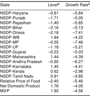
Table 5: ADF Tests of Variables
State Levela Growth Rateb
NSDP-Haryana –0.61 –5.84 NSDP-Punjab –1.71 –5.05 NSDP-Rajasthan –1.40 –5.85 NSDP-Bihar –2.16 –5.13 NSDP-Orissa –2.18 –7.41
NSDP-WB 1.84 –4.22
NSDP-MP –0.55 –7.46 NSDP-UP –1.18 –5.21 NSDP-Gujarat –0.23 –5.03 NSDP-Maharashtra 1.44 –4.39 NSDP-Andhra Pradesh –0.90 –6.27 NSDP-Karnataka 1.45 –4.41 NSDP-Kerala 0.62 –2.98 NSDP-Tamil Nadu 0.91 –3.85 Relative Price of Food –2.40 –5.46 Net Domestic Product 1.76 –4.05
M3/P 1.92 –4.56
a Equation includes an intercept and time trend. b Equation includes an intercept term.
This provides us with the following struc-ture of A, viz,
1 1 1 1
0 1 1 1
0 1 1 0
0 0 0 1
Unit Root Tests
In order to avoid spuriousness, the variables used in the estimation process need to be stationary. Table 5 reports the results of the augmented Dickey-Fuller (ADF) unit root tests applied to the levels and first differences of the system’s vari-ables. As Table 5 shows, all the variables are found to be I(1). Hence, the framework as described in (1) has been taken in growth rates.
Empirical Estimates
The obvious question that arises is: how can one measure the effectiveness of monetary policy in a particular state? Since all the variables are taken in real terms, monetary policy is postulated to be more effective in a state where the monetary shocks explain a larger proportion of output variance of that state. Given the annual data series employed in the study, we examined the 5-year ahead forecast error variance decomposition (FEVD) of g(Yi)’s,
and compared the proportion of FEVD of g(Yi) that are explained by monetary shock. An interesting pattern emerged when we delved into these numbers. Clearly, there is a clustering around of the states into two groups, the former in which monetary policy has higher impulses, and the latter, in which it was (relatively speaking) lower. This impact of the monetary shock is summarised in Tables 6 and 7, respectively for these two sets of states. Table 6 shows the states where monetary shocks have a less significant role in explaining state-wise output variance; the opposite is the case depicted in Table 7.
As evident, not all states respond to the same extent to a common monetary policy shock. In Table 6, the impact of a monetary policy shock is generally found to be high in the first year for states such as Uttar Pradesh and Madhya Pradesh; for all states, state NSDP generally declines during the first year following the policy shock and increases thereafter. The impulse responses indicate that unanticipated monetary policy shocks typically have their maximum impact on NSDP after three years. For
example, a policy innovation results in 6.83 per cent increase in NSDP in Punjab in the second year. The effect of the policy shock then builds to a maximum of 7.13 per cent in the fourth year and dies down thereafter.
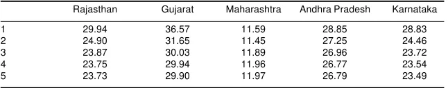
Table 7, on the other hand, depicts the reverse scenario where the impact of a policy shock on statewise output vari-ance is significant. As evident, most of the states included therein respond quite significantly to the policy innovation. For instance, the policy shock results in a substantial rise in NSDP in Andhra Pradesh in year 1, but subsequently dampens to 26.79 per cent by the end of the fifth year. Of these five states, Gujarat shows the most significant re-sponse to the policy shock with a high of 36.57 per cent; the lowest being for Maharashtra with 11.59 per cent. Inter-estingly, for most of these states, the effect of the policy shock is maximum in the first year; the exception being Maharashtra, which shows the maxi-mum response in the fifth year.
How far are these results in line with the stylised facts alluded to earlier? While there is an element of subjectivism in the clustering criterion in the sense that there is no statistical testing of the differences in output variance explained by mone-tary shock in state i vis-à-vis state j, the distinct pattern of clustering and the output variance between the two sets of states is, more or less, in line with the expected structural differences among the states. There are, however, certain exceptions to the observed attributes for certain states. This needs to be further explored.
V
Concluding Observations
The present paper employs time-series techniques to examine whether monetary policy had symmetric effects across major states in India during the period 1969-70 to 1998-99. The impulse response func-tions from an estimated SVAR reveal a core of states responding to monetary policy in a pro-active fashion than several other states. The study attempted to identify these core (and non-core) states that were more (less) sensitive to such policy shocks. Combining this with the earlier informa-tion on the concentrainforma-tion of manufactur-ing and the degree of financial deepenmanufactur-ing across states, it is clear that those states which have a greater concentration of manufacturing units or are relatively in-tensively banked tend to be more respon-sive to such shocks.
[image:6.567.204.526.536.598.2]The analysis began by setting out the basic facts on 14 Indian states, related to those aspects likely to give rise to shock asymmetry, viz, industry-mix, industrial concentration and financial deepening. A SVAR model was elaborated with a view to examining the impact of monetary policy innovations on output in each state. Based on our analysis, states were classified into two categories: (i) those significantly af-fected by monetary policy shocks (Type I states); and (ii) those where monetary policy is relatively less effective (Type II states). Our conclusions lend support to what our earlier theoretical discussion leads us to expect, viz, broadly speaking, states with a heavy concentration of manu-facturing enterprises and greater financial deepening tend to be more sensitive to
Table 6: States Where Monetary Shocks Have Less Significant Role in Statewise Output Variance: Proportion of Statewise Output Variance Explained by
Monetary Shocks
(Per cent)
Year Haryana Punjab UP Bihar Orissa WB MP Kerala TN
[image:6.567.205.528.633.697.2]1 0.76 1.95 6.72 0.26 0.01 3.23 4.61 1.10 0.03 2 2.35 6.83 4.65 2.03 0.02 4.78 2.90 2.11 0.30 3 2.51 7.00 4.61 2.22 0.04 7.38 3.45 2.12 0.52 4 2.52 7.13 4.71 2.22 0.04 7.30 3.51 2.10 0.52 5 2.58 7.11 4.71 2.22 0.04 7.29 3.53 2.12 0.55
Table 7: States Where Monetary Shocks Have a Significant Role in Statewise Output Variance: Proportion of Statewise Output Variance Explained by Monetary Shocks
(Per cent)
Rajasthan Gujarat Maharashtra Andhra Pradesh Karnataka
1 29.94 36.57 11.59 28.85 28.83
2 24.90 31.65 11.45 27.25 24.46
3 23.87 30.03 11.89 26.96 23.72
4 23.75 29.94 11.96 26.77 23.54
5 23.73 29.90 11.97 26.79 23.49
monetary policy shocks than relatively under-banked/less industrialised states. There are, however, certain exceptions to the observed attributes of some of the states. This raises the possibility that different states are subject to shocks, which are asymmetric and hence, that in a sense, the Indian federal economy is an incomplete currency area. Monetary policy may then be more responsive to the shocks occur-ring in certain states, and while smooth-ening out output fluctuations in this group of states, might be leaving other types of shocks occurring in the remaining states, largely unattended. Further investigation is of course, necessary to confirm the presence and extent of such asymmetries as well as examine in detail their sources. If it does turn out that the regional asym-metries are indeed significant with the Indian federation falling well short of an optimum currency area, then institutional changes of a far-reaching kind in the monetary policy mechanism would be called for. While it may be premature to speculate on the nature of the required changes, there is no gainsaying that in view of severe resource constraints faced by several Indian states [Rao 2002], monetary policy would need to take regional perspective into account.
Address for correspondenc:
Notes
[The views expressed in the paper are the authors’ own, and not necessarily those of the institutions to which they belong. The authors would like to thank, without implicating M D Patra for his insightful comments on an earlier draft.]
1 See for example, Singh et al (1982), Jadhav (1994), Rangarajan (1988), Rangarajan and Arif (1990) and Reddy (2002).
2 These regions are New England, Mid-east, Great Lakes, Plains, Southeast, Southwest, Rocky Mountain and Far West.
3 The sample coincides with Ahluwalia’s set of 14 states for the sake of comparing the SDP among Indian states [Ahluwalia 2000]. 4 The data has been culled out from the Database
of the Indian Economy (H L Chandok), National Accounts Data (Central Statistical Organisation) and the Handbook of Statistics on Indian Economy (Reserve Bank of India). 5 Both state-specific NSDP’s and economywide
NDP have been taken at factor cost at constant prices.
References
Ahluwalia, M S (2000): ‘Economic Performance of States in the Post-Reform Period’, Economic and Political Weekly, May, 1637-48. Bagchi, A, J L Bajaj and W A Byrd (1992): State
Finances in India, Vikas Publishing House, New Delhi.
Bayoumi, T and B Eichengreen (1993): ‘Shocking
Aspects of European Monetary Integration’ in F Torres and F Giavazzi (eds), Adjustment and Growth in the European Monetary Union, Cambridge University Press.
Bernanke, B and A Blinder (1988): ‘Money, Credit and Aggregate Demand’, American Economic Review: Papers and Proceedings, 435-39. Carlino, G and R Defina (1998): ‘The Differential
Regional Effects of Monetary Policy’, Review of Economics and Statistics, 34: 572-87. – (1999): ‘The Differential Effects of Monetary
Policy: Evidence from the US States’, Journal of Regional Science, 39: 339-58.
Chaudhuri, S (2000): ‘Economic Growth in the States-Four Decades-I’, ICRA Bulletin: Money and Finance, October-December, 45-69. Dasgupta, D, P Maiti, R Mukherjee, S Sarkar and
S Chakrabarti (2000): ‘Growth and Inter-state Disparities in India’, Economic and Political Weekly, July, 2413-22.
Dornbusch, R, C A Favero and F Giovazzi (1998): ‘The Immediate Challenges for the European Central Bank’, NBER Working Paper No 6369. Garrison, C B and H S Chang (1979): ‘The Effects of Monetary Forces in Regional Economic Activity’, Journal of Regional Science, 19: 15-29.
Garrison, C B and J R Kort (1983): ‘Regional Impact of Monetary and Fiscal Policy: A Comment’, Journal of Regional Science, 23: 249-61.
Gerlach, S and F Smets (1995): ‘The Monetary Transmission Mechanism: Evidence from the G-7 Countries’, CEPR Discussion Paper No 1219.
Jadhav, Narendra (1994): Monetary Economics for India, McMillan India.
Kashyap, A and J C Stein (1997): ‘The Role of Banks in Monetary Policy: A Survey with Impli-cations for the European Monetary Union’,
Federal Reserve Bank of Chicago Economic Perspectives, September/October, 2-18. Kurian, N J (2000): ‘Widening Regional Disparities
in India: Some Indicators’, Economic and Political Weekly, February, 538-50. Miller, R J (1978): The Regional Impact of
Monetary Policy in the US, Lexington DC. Ramaswamy, R and T Sloek (1997): ‘The Real Effects of Monetary Policy in the European Union: What Are the Differences’, IMF Working Paper No 160, IMF, Washington. Rangarajan, C (1988): ‘Issues in Monetary
Management’, Presidential Address, 71st Conference of Indian Economic Association. Rangarajan, C and R Arif (1990): ‘Money, Output and Prices: A Macroeconometric Model’,
Economic and Political Weekly, April. Rao, M G (2002): ‘State-Level Fiscal Reforms in
India’, Paper presented at the Conference on Comparative Economic Development, Cornell University.
Reddy, Y V (2002): ‘Parameters of Monetary Policy in India’, 88th Annual Conference of Indian Econometric Society.
Shand, R and S Bhide (2000): ‘Sources of Economic Growth: Regional Dimensions of Reforms’, Economic and Political Weekly, October, 3747-57.
Sims, C (1980): ‘Macroeconomics and Reality’,
Econometrica, 48: 1-48.
Singh, A P, S L Shetty and T R Venkatachalam (1982): ‘Monetary Policy in India: Issues and Evidence’, Supplement to RBI Occasional Papers.
Taylor, L L and M K Yucel (1996): ‘The Policy Sensitivity of Industries and Regions’, Working Paper No 12, Federal Reserve Bank of Dallas. Venkataraman, K (1968): States’ Finances in India, George Allen and Unwin, London.