Linear Partial Differential Equations of First Order as Bi Dimensional Inverse Moments Problem

http://dx.doi.org/10.4236/am.2015.66090

Linear Partial Differential Equations of

First Order as Bi-Dimensional Inverse

Moments Problem

Maria Beatriz Pintarelli

Facultad de Ingenieria, Universidad Nacional de La Plata, La Plata, Argentina Email: [email protected]

Received 29 March 2015; accepted 30 May 2015; published 2 June 2015

Copyright © 2015 by author and Scientific Research Publishing Inc.

This work is licensed under the Creative Commons Attribution International License (CC BY). http://creativecommons.org/licenses/by/4.0/

Abstract

We consider linear partial differential equations of first order

( ) ( ) ( ) ( )

x t

( ) ( ) ( )

a x t w, x t, +b x t w, x t, =h x t w x t, , +r x t, on a region E=

(

a b1, 1

) (

× a b2, 2

)

. We will see

that we can write the equation in partial derivatives as an Fredholm integral equation of the first kind and will solve this latter with the techniques of inverse problem moments. We will find an approximated solution and bounds for the error of the estimated solution using the techniques on problem of moments.

Keywords

Linear PDEs, Freholm Integral Equations, Generalized Moment Problem

1. Introduction

We consider linear partial differential equation of first order of the general form:

( ) ( ) ( ) ( ) ( ) ( ) ( )

, x , , t , , , ,

a x t w x t +b x t w x t =h x t w x t +r x t (1) where the unknown function w x t

( )

, is defined in E=

(

a b1, 1

) (

× a b2, 2

)

. We will consider Dirichlet conditions

on the boundary S= ∂E and a x t

( )

, , b x t

( )

, , h x t

( )

, and r x t

( )

, are known functions. Equation (1) is a particular case of the quasi-linear equation

(

) ( ) (

) ( )

(

)

1

( )

, , x , , , t , , , , , .

a x t w w x t +b x t w w x t =h x t w a b h∈C E

above equation. This equation expresses that the tangent to a curve on the surface z=w x t

( )

, is proportional to

(

a b h, ,

)

. The solution of the quasi-linear equation can therefore be expressed by

(

)

(

)

(

)

d d d

, , , , , ,

d d d

x t z

a x t w b x t w h x t w

s = s= s= (2)

where r s

( ) ( )

=x s iˆ+t s j

( )

ˆ+z s k

( )

ˆ is a parametric curve belonging to the solution surface. Then we must solve a system of three simultaneous differential equations of the first order.

The general solution of this system of three equations consists of families of curves which are described by a system of three parametric equations with three arbitrary constants determined by initial conditions. This system is generally not linear and it is known that a system of non linear ordinary differential equations is difficult to solve explicitly. In general, geometrically in R3, the curves are determined by at least two intersecting surfaces transversely. This can be accomplished, for example, eliminating the parameter s and obtain

(

)

(

)

1 , , 1 2 , , 2

w x t w =c w x t w =c (3) where c₁ and c₂ are arbitrary constants. The general solution will be

( )

2 1

w =

ϕ

w (4) where ϕ is an arbitrary function of w₁. For a particular solution you can find the function ϕ de modo que

( )

2 1

w =

ϕ

w so to satisfy f x t z1

(

, ,

)

=0 y f2

(

x t z, ,

)

=0.

We will show that, the partial differential Equation (1) can be transformed into a integral equation and that this one can be numerically solved using techniques normally employed with generalized moment problems [1]-[3]. This approach was already suggested by Ang [4] in relation with the heat conduction equation and we have applied to the non linear Klein-Gordon equation [5].

Next section is devoted to show how the differential Equation (1) is transformed into integral equation of first kind that can be seen as generalized moments problem as is shown in Section 3. There we also proof a theorem that guarantees under certain conditions the stability and convergence of the finite generalized moment problem. In Section 4, we exemplify the general method by applying it to some linear PDEs which are particular cases of Equation (1). Finally in Section 5, the method is applied to solve an equation of Klein Gordon with boundary conditions in a rectangular region.

The d-dimensional generalized moment problem [1] [2] can be posed as follows: find a function u on a domain Ω ⊂Rd satisfying the sequence of equations

( ) ( )

_n d _n

u x g x x µ n

Ω = ∈

∫

N (5)

where

( )

g_n is a given sequence of functions lying in L2

( )

Ω linearly independent. Many inverse problems can be formulated as an integral equation of the first kind, namely,

( ) ( )

, d

( )

( )

, b

aK x y u y y= f x x∈ a b

∫

( )

,

K x y and f x

( )

are given functions and u y

( )

is a solution to be determined, f x

( )

is a result of experimental measurements and hence is given only at finite set of points. It follows that the above integral equation is equivalent to the following moment problem

(

,

) ( )

d

( )

1, 2, b

n n

aK x y u y y= f x n=

∫



Also we consider the multidimensional moment problems

(

_n,

)

( )

d

( )

_n 1, 2, , d.

K x y u y y f x n

Ω = = Ω ⊂

∫

 R

Moment problem are usually ill-posed [6] [7]. There are various methods of constructing regularized solutions, that is, stable appoximate solutions with respect to the given data μn. One of them is the method of truncated

expansion [4].

The method of truncated expansion consists in approximating (5) by finite moment problems

( ) ( )

_i d _i 1, 2, , .

u x g x x µ i n

Ω = =

Solved in the subspace g g1, 2,,gn generated by g g1, 2,,gn (6) is stable. Considering the case where

the data

µ

=

(

µ µ

1, 2,,

µ

n

)

are inexact, we apply some convergence theorems and error estimates for the

regularized solutions.

2. Linear Partial Differential Equations of First Order as Integral Equations of First

Kind

Let F w x t

(

( )

,

)

=0 be a partial differential equations such as (1). The solution w x t

( )

, is defined on the re- gion E=

(

a b1, 1

) (

× a b2, 2

)

and verifies Dirichlet conditiones on the boundary C= ∂E:

( )

1, 1

( )

( )

1, 2

( )

w a t =s t w b t =s t

(

, 2

)

3

( )

(

, 2

)

4

( )

w x a =s x w x b =s x

Let F∗ =

(

F w F w₁

( ) ( )

, ₂

)

be a vectorial field such that w verifies div F

( )

∗ =h∗

( )

w with h∗ a known function and, reciprocally, if w verifies div F

( )

∗ =h∗

( )

w then F w x t

(

( )

,

)

=0.

Let u x t

(

, , ,

τ ξ

)

be the auxiliary function such that

(

)

(

)

(

1 , , , , 2 , , ,

)

.

u uk x tτ ξ uk x tτ ξ

∇ =

Since

( )

( )

udiv F∗ =uh∗ w

we have

( )

d

( )

d .

Eudiv F A Euh w A

∗ ₌ ∗

∫∫

∫∫

Moreover, as

( )

( )

udiv F∗ =div uF∗ −F∗⋅∇u

and

( )

( )

( )

d

d d d

C

E E E

uF n s

udiv F A div uF A F u A

∗

∗ ∗ ∗

=_∫ ⋅

= − ⋅∇

∫∫

∫∫

_{}

∫∫

we obtain

( )

d

( )

d d

Euh w A C uF n s EF u A

∗ ₌ ∗ _{⋅ −} ∗_⋅∇

∫∫

∫

∫∫

(7)

where ∇ =u

(

u uτ, ξ

)

. Then (7) gives:

( )

d d

( )

d

Euh w A EF u A C uF n s

∗ ₊ ∗_{⋅∇ =} ∗ _⋅

∫∫

∫∫

∫

and

( )

d d

(

( )

)

d

(

( )

1 2

)

d .

Euh w A EF u A E uh w F u A E uh w F uτ F uξ A

∗ ₊ ∗_{⋅∇ =} ∗ ₊ ∗_{⋅∇ =} ∗ _{+ +}

∫∫

∫∫

∫∫

∫∫

Then

( )

(

( )

)

(

)

( )

1 2 1 2

2

=1

, , , , d d ,

b b

i i

a a

i

u h_ ∗ w + F w τ ξ k x tτ ξ _ ξ τ =G x t



∑



∫ ∫

(8)

where

( )

(

(

)

(

(

)

)

(

)

(

(

)

)

)

(

)

(

(

)

)

(

)

(

(

)

)

(

)

2 2 1 1

1 1 1 1 1 1

2 2 2 2 2 2

, , , , , , , , , d

, , , , , , , , d .

b

a b

a

G x t u x t b F w b u x t a F w a

u x t b F w b u x t a F w a

ξ ξ ξ ξ ξ

τ τ τ τ τ

= −

+ −

∫

∫

( ) ( ) ( ) ( ) ( ) ( ) ( )

, , , , , , , .

a

τ ξ

w_τ

τ ξ

+b

τ ξ

w_ξ

τ ξ

=h

τ ξ

w

τ ξ

+r

τ ξ

We take as vector field

( )

( )

(

1 , 2

)

(

( ) ( ) ( ) ( )

, , , , ,

)

F∗= F w F w = aτ ξ w τ ξ b τ ξ w τ ξ

and

(

_{, , ,}

)

_em x1( 1)( 1)_e m2( )(t 1 1)

u x tτ ξ = − + τ+ − + ξ+

where m₁ y m₂ are arbitrary constants. Then

( )

(

( ) ( )

)

(

( ) ( )

)

( )

, , , ,

.

div F a w b w

aw bw a w b w hw r a w b w h w

τ ξ

τ ξ τ ξ τ ξ

τ ξ τ ξ τ ξ τ ξ

∗

∗

= +

= + + + = + + + =

Therefore, Equation (8) yields

(

)

(

)

(

)

( )

1 2 1 2

1 2 1 2 1 2

1 1 d d , d d .

b b b b

a a uw h a+ τ + −bξ m x+ a m t− + b

ξ τ

=G x t − a a ur

ξ τ

∫ ∫

∫ ∫

(9)

3. Solution of Generalized Moment Problems

If (9) can be written in the form:

( )

(

)

(

)

( )

1 2 1 2

, , , , d d ,

b b

a a F w

τ ξ

K x t

τ ξ τ ξ ϕ

= x t

∫ ∫

with

ϕ

( )

x t, ∈L E2

( )

, then taking a basis

{

_m

( )

,

}

m

x t

ψ of L E2

( )

this Fredholm integral equation of first kind can be transformed into a bi-dimensional generalized moment problem

( )

(

)

( )

1 2 1 2

, , d d 0,1, 2,

b b

m m

a a F w

τ ξ

K

τ ξ τ ξ µ

= m=

∫ ∫

 (10)

where

( )

1 2

(

) ( )

1 2

, b b , , , , d d

m _{a a} m

K

τ ξ

=

∫ ∫

K x t

τ ξ ψ

x t x t (11) and the moments µ_m are

( ) ( )

1 2 1 2

, , d d .

b b

m _{a a} x t m x t x t

µ

=

_{∫ ∫}

ϕ

ψ

(12)

If the functions

{

_m

(

,

)

}

m

K τ ξ are linearly independent then the generalized moment problem defined by Equations (10), (11) and (12) can be solved considering the correspondent finite problem

( )

(

)

( )

1 2 1 2

, , d d 0,1, 2, ,

b b

m m

a aF w

τ ξ

K

τ ξ τ ξ µ

= m= n n∈N

∫ ∫

 (13)

whose solution we denote p_n

( )

τ ξ, ≈β τ ξ

( )

, =F w

(

( )

τ ξ,

)

. If F w

( )

has continuous inverse, then 1

(

( )

)

( )

, ,

n n

F− p τ ξ =w τ ξ is an estimation of w

( )

τ ξ

, . To reach this result let consider the basis

{

(

)

}

0 ,

i _i

φ τ ξ ∞₌ obtained from the sequence

{

(

)

}

0 , n

m _m

K τ ξ ₌ by Gram-Schmidt method and addition of the necessary functions in order to have an orthonormal basis.

We then approximate the solution β τ ξ

(

,

)

=F w

(

(

τ ξ,

)

)

de (13) with

( )

( )

0

, ,

n

n i i

i

p τ ξ λ φ τ ξ

=

=

∑

with

0

0,1, , i

i ij j

j

C i n

λ µ

=

=

∑

= _

( )

( ) ( )

( )

( )

1 1 2 , ,

1 , 1 ; 1

, i

i k

ij kj i

k j

k

K

C τ ξ φ τ ξ C φ τ ξ i n j i

φ τ ξ

− ₋

=

 

 

= − ⋅ < ≤ ≤ <

 



∑



(14)

(

)

1

, 0,1, , .

ii i

C = φ τ ξ − i=  n (15) We extend to the bi-dimensional case the arguments of reference [8] [9] and we have the following.

Theorem 1. Let

{ }

0 n

m m

µ ₌ be a set of real numbers and let ε and E be two positive numbers such that

( ) ( )

2 1 2 1 2 2 0

, , d d

n _{b b}

m m

a a

m

K τ ξ β τ ξ τ ξ µ ε

=

− ≤

∑ ∫ ∫

(16)

y

(

)

(

)

2 1 2 1

2 2 2 2 2

1 1 2 2 d d

b b

a a b a

β

τ b a

β

ξ

τ ξ

E

 _{− + −}  _≤  

∫ ∫

then

( )

(

)

2 1 2 1 2

2 _{T 2}

2

, d d min ; 0,1, ,

8 1

b b

a a n

E

CC n N

n

β τ ξ τ ξ≤  ε + = 

+

 

 

∫ ∫

 (17)

whereC is the triangular matriz with elements C_ij

(

1< ≤i n;1≤ <j i

)

. And

( )

( )

(

)

2 1 2 1 2

2 _{T 2}

2

, , d d .

8 1 b b n a a E p CC n

τ ξ −β τ ξ τ ξ≤ ε + +

∫ ∫

(18)

Si F−1

( )

x is Lipschitz in R2, ie if 1

( )

1

( )

F− x −F− y ≤λ x−y for some λ and ∀

( )

x y, ∈R2 then

( )

( )

(

)

2 1 2 1

2

2 _{T 2}

2

, , d d .

8 1

b b n a a

E

w w CC

n

τ ξ − τ ξ τ ξ λ≤  ε + 

 ₊ 

 

∫ ∫

(19)

Proof. The demonstration is similar to that we have done for the unidimensional generalized moment problem [8], which is based in results of Talenti [10] for the Hausdorff moment problem. Here we simply introduce the necessary modification for the bi-dimensional case.

Without loss of generality we take

{

}

0 0 n

m m

µ = ₌ in (16). We write

( )

, hn

( )

, tn

( )

,

β τ ξ

=

τ ξ

+

τ ξ

where hn

( )

τ ξ

, is the orthogonal projection of

β τ ξ

( )

, on the linear space that the set

{

(

,

)

}

₀

n

m _m

K τ ξ ₌ gene- rates and tn

( )

τ ξ

, =

β τ ξ

( )

, −hn

( )

τ ξ

, is the orthogonal projection of

β τ ξ

( )

, on the orthogonal complement.

In terms of the basis

{

(

)

}

0 ,

i _i

φ τ ξ ∞₌ the functions hn

( )

τ ξ

, and tn

( )

τ ξ

, reads

( )

( )

( )

( )

0 1

, , ; , ,

n

n i i n i i

i i n

h τ ξ λ φ τ ξ t τ ξ λ φ τ ξ

∞ = = + =

∑

=

∑

with 0 0,1, i

i ij j

j

C i

λ µ

=

=

∑

= _

and the matrix elements C_ij given by (14) and (15). In matricial notation:

1 1 2 2 . n n C λ µ λ µ

λ µ λ µ

Besides

( ) ( )

( ) ( )

2 1 2 1

2 1 2 1

, , d d y , , d d .

b b b b

i _{a a} i i _{a a} Ki

λ

=

_{∫ ∫}

β τ ξ φ τ ξ τ ξ

µ

=

_{∫ ∫}

β τ ξ

τ ξ τ ξ

Therefore

( )

2 1 2 1

2 T T 2 T 2

, d d , , .

b b

n

a a h

τ ξ

τ ξ

=

λ λ

= C C

µ µ

≤ C C

µ

≤ C C

ε

∫ ∫

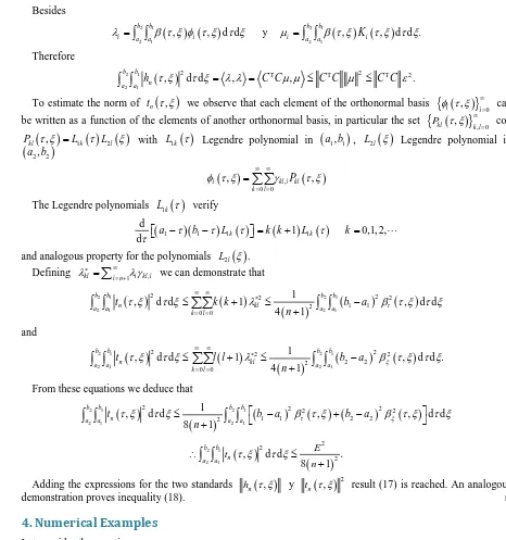
To estimate the norm of tn

( )

τ ξ

, we observe that each element of the orthonormal basis

{

φ τ ξi

(

,

)

}

_{i 0} ∞

= can be written as a function of the elements of another orthonormal basis, in particular the set

{

( )

}

, 0 , kl _{k l}

P τ ξ ∞₌ con

( )

, 1

( ) ( )

2

kl k l

P

τ ξ

=L

τ

L

ξ

with L_1k

( )

τ

Legendre polynomial in

(

a b₁, ₁

)

, L_2l

( )

ξ

Legendre polynomial in

(

a b2, 2

)

( )

,

( )

0 0

, ,

i kl i kl

k l

P

φ τ ξ ∞ ∞γ τ ξ

= =

=

∑∑

The Legendre polynomials L_1k

( )

τ

verify

(

1

)(

1

) ( )

1

(

) ( )

1 d

1 0,1, 2,

dτ a −τ b −τ Lk τ =k k+ Lk τ k=  and analogous property for the polynomials L₂l

( )

ξ

.

Defining _,

1 kl i n i kl i

λ∗ ∞ λ γ

= +

=

∑

we can demonstrate that

( )

(

)

(

)

(

)

( )

2 1 2 1

2 1 2 1

2 2 2 2

1 1

2 0 0

1

, d d 1 , d d

4 1

b b b b

n kl

a a a a

k l

t k k b a

n τ

τ ξ

τ ξ

∞ ∞

λ

∗

β τ ξ τ ξ

= = ≤ + ≤ − +

∑∑

∫ ∫

∫ ∫

and

( )

(

)

(

)

(

)

( )

2 1 2 1

2 1 2 1

2 2 2 2

2 2

2 0 0

1

, d d 1 , d d .

4 1

b b b b

n kl

a a a a

k l

t l l b a

n ξ

τ ξ

τ ξ

∞ ∞

λ

∗

β τ ξ τ ξ

= =

≤ + ≤ −

+

∑∑

∫ ∫

∫ ∫

From these equations we deduce that

( )

(

)

(

)

( ) (

)

( )

2 1 2 1

2 1 2 1

2 2 2 2 2

1 1 2 2

2 1

, d d , , d d

8 1

b b b b

n

a a t a a b a b a

n τ ξ

τ ξ

τ ξ

≤ _ −

β τ ξ

+ −

β τ ξ

_

τ ξ

+

∫ ∫

∫ ∫

( )

(

)

2 1 2 1 2 2 2

, d d .

8 1 b b n a a E t n

τ ξ τ ξ

∴ ≤

+

∫ ∫

Adding the expressions for the two standards h_n

( )

τ ξ, y tn

(

τ ξ,

)

2 result (17) is reached. An analogous demonstration proves inequality (18). □

4. Numerical Examples

Let consider the equation

0

x t

xtw +w =

in the domain E=

( ) ( )

0, 2 × 0, 2 and boundary condition on ∂E given by

( )

2₂

( )

2₂

0, e t 2, 3et

w t = − w t = −

( ) (

)

( ) (

)

2

, 0 1 , 2 1 e

w x = +x w x = +x −

The exact solution is _{w x t}

( ) (

_, = _x+_{1 e}

)

−t22_.

In Figure 1(a) the approximate numerical solution (dark gray) and the exact one (light gray) are compared. Was taken

ψ

ij

( )

x t, =x ti j with i=0,1, 2 and j=0,1, 2.

[image:6.595.67.533.82.579.2]

[image:7.595.189.415.229.310.2]

(a) (b)

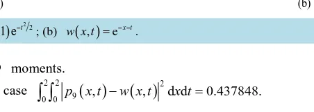
Figure 1. (a) _{w x t}

( ) (

_, = _x+_{1 e}

)

−t22

; (b)

( )

, ex t

w x t = − − .

Thus were taken n=9 moments.

The accuracy is, in this case 2 2 ₉

( )

( )

2

0 0 p x t, −w x t, d dx t=0.437848.

∫ ∫

Let consider the equation

(

2

)

(

2

)

(

(

) (

)

)

1

x t

xt+t w + x +t w = − t + +t x t+x w

in the domain E=

( ) ( )

0,3 × 0,3 and boundary condition on ∂E given by

( )

( )

3

0, et 3, e t

w t = − w t = − −

( )

( )

3

, 0 e x , 3 e x

w x = − w x = − −

The exact solution is

( )

, e x t.

w x t = − −

In Figure 1(b) the approximate numerical solution (dark gray) and the exact one (light gray) are compared. Was taken

( )

, i j

ij x t x t

ψ

= with i=0,1, 2 and j=0,1, 2.

And m₁ =m₂ =1 in u.

Thus were taken n=9 moments.

The accuracy is, in this case 3 3 ₉

( )

( )

2

0 0 p x t, −w x t, d dx t=0.333021.

∫ ∫

5. Application

We want to find w x t

( )

, ∈L E2

( )

with E=

(

a b₁, ₁

) (

× a b₂, ₂

)

such that satisfies the Klein-Gordon equation

( )

,

( )

,

(

( )

,

)

( )

,

xx tt

w x t −w x t =h w x t +r x t (20)

where h y r are known functions. And boundary conditions

( )

1, 1

( )

( )

1, 2

( )

w a t =g t w b t =g t

(

, 2

)

3

( )

(

, 2

)

4

( )

w x a =g x w x b =g x

we write

(

,

)

(

,

)

(

(

,

)

)

(

,

)

.

wττ τ ξ −wξξ τ ξ =h w τ ξ +r τ ξ (21)

We take as vector field

( )

( )

(

1 , 2

)

(

( )

, ,

( )

,

)

F∗= F w F w = wτ τ ξ −wξ τ ξ

and

(

)

( 1)( 1) ( )(1 1)

, , , e x e t .

Then

( )

( )

,

div F∗ =wττ−wξξ =h∗ τ ξ

where

( )

,

(

( )

,

)

( )

, .

h∗ τ ξ =h wτ ξ +r τ ξ

Since

( )

( )

udiv F∗ =uh∗ w

we have

( )

d

( )

d .

Eudiv F A Euh w A

∗ ₌ ∗

∫∫

∫∫

Moreover, as

( )

( )

.

udiv F∗ =div uF∗ −F∗⋅∇u

Therefore

( )

d

( )

d d

Eudiv F A Ediv uF A EF u A

∗ ₌ ∗ ₋ ∗_⋅∇

∫∫

∫∫

∫∫

(22)

in addition

( )

d

(

(

)

( )

)

( )

d

(

)

d

Ediv uF A E uwτ τ uwξ ξ Eudiv F A E u wτ τ u wξ ξ A

∗ _{= − =} ∗ _{+ −}

∫∫

∫∫

∫∫

∫∫

(23)

then (22) and (23) we obtain:

(

)

d d .

EF u A E u wτ τ u wξ ξ A

∗_{⋅∇ = −}

∫∫

∫∫

(24)

Also doing integration by parts is reached:

( )

( )

(

(

) (

2

)

2

)

, , 1 1 d

EF udA A x t B x t Euw x t A

∗_{⋅∇ = + − + − +}

∫∫

∫∫

(25)

with

( )

(

(

) (

)

(

) (

)

)

( )

(

(

) (

)

(

) (

)

)

2 2 1 1

1 1 1 1

2 2 2 2

, , , , , , , , , d

, , , , , , , , , d .

b

a b

a

A x t w b u x t b w a u x t a

B x t w b u x t b w a u x t a

τ τ

ξ ξ

ξ ξ ξ ξ ξ

τ τ τ τ τ

= −

= −

∫

∫

From (23), (24) and (25) and after several calculations:

( )

( )

2 1

(

) (

)

(

)

(

)

2 1

2 2

, , b b 1 1 1 1 d d .

a a

A x t +B x t =

∫ ∫

u w_ _ x+ − +t _+wτ − −x +wξ +t _ x t

If t=x then

( )

( )

( )

2 1

(

)

2 1

, , b b 1 d d .

a a

t A t t B t t u t wτ wξ x t

ϕ

= + =

_{∫ ∫}

+ _− + _ (26)

We write (26) as:

( )

(

)

22 11 ( )( )

1 2

e d d .

1

b b _t

a a

t

w w x t

t

τ ξ

τ ξ

ϕ

₌ − + + + _{− + }

 

+

∫ ∫

(27)

We can see that (27) is an integral equation of the form

( ) (

)

( )

1 2 1 2

, , , d d

b b

a a w

τ ξ

K t

τ ξ τ ξ ϕ

t

∗ ₌ ∗

∫ ∫

where the unknown function is w∗

( )

τ ξ

, = − +w_τ w_ξ, the kernel is

(

)

( )(1 2) , , e t

K tτ ξ = − + τ ξ+ + and

( )

₍

( )

₎

.

1

t t

t

ϕ

ϕ

∗ ₌

To solve (27) as a problem of two-dimensional moments we apply seen in Section 3 and we obtain an approximation pn

( )

τ ξ

, to −wτ +wξ.

Now we solve the partial differential equation of the first order

( )

,

w_τ w_ξ r

τ ξ

− + = (28)

where r

( )

τ ξ

, = p_n

( )

τ ξ

, , a

( )

τ ξ

, = −1, b

( )

τ ξ

, =1 y h

( )

τ ξ

, =0. To find the solution of the Equation (28) algorithm of Section 3 applies.

Numerical Examples

We want to find w x t

( )

, ∈L E2

( )

with E=

( ) (

0, 2 × 0,∞

)

such that satisfies the Klein-Gordon equation

( )

( )

(

)

( )

( )2

1 2

, , 4 8 1 , 2e x t

tt xx

w x t −w x t = t + +t w x t + − − + (29)

with boundary conditions

( )

( )2

_{( )}

( )2

1 2 1

0, e t 2, 3e t 0

w t = − + w t = − − + t>

( ) (

, 0 1 e ,

)

x 0 2.

w x = x+ − < <x

The exact solution is

( ) (

)

( )12

, 1 e x t

w x t = x+ − − + .

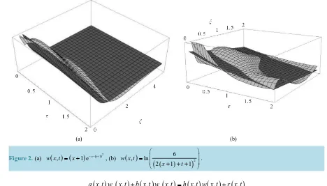
In Figure 2(a) the approximate numerical solution (dark grey) and the exact one (light grey) are compared. For the first step was taken the base

ψ

i

( )

t tiet

−

= with i=0,1,,8 and as an auxiliary function

(

)

(1 ) (1 ) , , , e x t

u x tτ ξ = − + −ξ +τ . For the second step was taken the base

ψ

ij

( )

x t, x ti je x t

− −

= with i=0,1, 2 and

0,1, 2.

j=

And

(

)

( 1 1)( ) 0.5( )(1 1 )

, , , e x t

u x tτ ξ = − + + −ξ + +τ in order to avoid discontinuities. Thus were taken n=9 moments.

The accuracy is, in this case 2 ₉

( )

( )

2

0 0 p x t, w x t, d dx t 0.0997437. ∞

− =

∫ ∫

We want to find w x t

( )

, ∈L E2

( )

with E=

( ) ( )

0, 2 × 0, 2 such that satisfies the Klein-Gordon equation

( )

,

( )

, ew

tt xx

w x t −w x t = − (30) with boundary conditions

( )

(

)

2

( )

(

)

2

6 6

0, ln 2, ln

3 7

w t w t

t t

   

   

= _{ } = _{ }

+ +

   

( )

(

)

(

)

2

( )

(

(

)

)

2

6 6

, 0 ln , , 2 ln

2 1 1 2 1 3

w x w x

x x

   

   

= =

 _{+ +}   _{+ +} 

   

The exact solution is

( )

(

)

(

)

2

6

, ln

2 1 1

w x t

x t

 

 

=

 _{+ + +} 

 

.

In Figure 2(b) the approximate numerical solution (dark grey) and the exact one (light grey) are compared. For the first step was taken the base

ψ

i

( )

t tiet

−

= with i=0,1,,8 and as an auxiliary function

(

)

(1 ) (1 ) , , , e x t

u x tτ ξ = − + −ξ +τ . For the second step was taken the base

ψ

ij

( )

x t, x ti je x t

− −

= with i=0,1, 2 and

0,1, 2.

j=

And u x t

(

, , ,τ ξ

)

=e− +(x1 1)(+ −ξ) 0.5( )(t+1 1+τ) in order to avoid discontinuities. Thus were taken n=9 moments.

The accuracy is, in this case 2 2 ₉

( )

( )

2

0 0 p x t, −w x t, d dx t=0.615126.

∫ ∫

6. Conclusions

[image:10.595.74.542.88.355.2]

(a) (b)

Figure 2. (a)

( ) (

)

( )12

, 1 ex t

w x t = x+ − − + , (b)

( )

(

)

(

)

2

6

, ln

2 1 1

w x t

x t

 

 

=

 _{+ + +} 

 

.

( ) ( ) ( ) ( ) ( ) ( ) ( )

, _x , , _t , , , ,

a x t w x t +b x t w x t =h x t w x t +r x t

on a region E=

(

a b₁, ₁

) (

× a b₂, ₂

)

can be written as an Fredholm integral equation

(

)

(

)

(

)

( )

1 2 1 2

1 2 1 2 1 2

1 1 d d , d d .

b b b b

a a uw h a+ τ + −bξ m x+ a m t− + b

ξ τ

=G x t − a a ur

ξ τ

∫ ∫

∫ ∫

(31)

If (31) can be written in the form:

( )

(

)

(

)

( )

1 2 1 2

, , , , d d ,

b b

a a F w

τ ξ

K x t

τ ξ τ ξ ϕ

= x t

∫ ∫

with

ϕ

( )

x t, ∈L E2

( )

, then taking a basis

{

ψm

( )

x t,

}

_m of

( )

2

L E this Fredholm integral equation of the first kind can be transformed into a bi-dimensional generalized moment problem

( )

(

)

( )

1 2 1 2

, , d d 0,1, 2,

b b

m m

a aF w

τ ξ

K

τ ξ τ ξ µ

= m=

∫ ∫

 (32)

where

( )

1 2

(

) ( )

1 2

, b b , , , , d d

m _{a a} m

K

τ ξ

=

∫ ∫

K x t

τ ξ ψ

x t x t (33) and the moments µ_m are

( ) ( )

1 2 1 2

, , d d .

b b

m _{a a} x t m x t x t

µ

=

_{∫ ∫}

ϕ

ψ

(34)

If the functions

{

_m

(

,

)

}

m

K τ ξ are linearly independent then the generalized moment problem defined by Equations (32), (33) and (34) can be solved considering the correspondent finite problem.

References

[1] Akheizer, N.I. (1965) The Classical Moment Problem. Olivier and Boyd, Edinburgh.

[2] Akheizer, N.I. and Krein, M.G. (1962) Some Questions in the Theory of Moment. American Mathematical Society. Providence.

[3] Shohat, J.A. and Tamarkin, J.D. (1943) The Problem of Moments. Mathematical Surveys, American Mathematical So-ciety, Providence. http://dx.doi.org/10.1090/surv/001

Theory and Heat Conduction. Lectures Notes in Mathematics, Springer-Verlag, Berlin. http://dx.doi.org/10.1007/b84019

[5] Pintarelli, M.B. and Vericat, F. (2012) Klein-Gordon Equation as a Bi-Dimensional Moment Problem. Far East Jour-nal of Mathematical Sciences, 70, 201-225.

[6] Tikhonov, A. and Arsenine, V. (1976) Méthodes de résolution de problèmes mal posés. MIR, Moscow. [7] Engl, H.W. and Groetsch, C.W. (1987) Inverse and Ill-Posed Problems. Academic Press, Boston.

[8] Pintarelli, M.B. and Vericat, F. (2008) Stability Theorem and Inversion Algorithm for a Generalized Moment Problem.

Far East Journal of Mathematical Sciences, 30, 253-274.

[9] Pintarelli, M.B. and Vericat, F. (2011) Bi-Dimensional Inverse Moment Problems. Far East Journal of Mathematical Sciences, 54, 1-23.

[10] Talenti, G. (1987) Recovering a Function from a Finite Number of Moments. Inverse Problems, 3, 501-517. http://dx.doi.org/10.1088/0266-5611/3/3/016

[11] Ames, W.F. (1992) Numerical Methods for Partial Differential Equations. Academic Press, New York.

[12] Lapidus, L. and Pinder, G.F. (1982) Numerical Solution of Partial Differential Equations in Science and Engineering. John Wiley and Sons, New York.

[13] Smith, G.D. (1985) Numerical Solution of Partial Differential Equations: Finite Difference Methods. Oxford Universi-ty Press, New York.