On Two Problems for Matrix Polytopes

(1)

http://dx.doi.org/10.4236/am.2014.517253

How to cite this paper: Yılmaz, Ş. and Büyükköroğlu, T. (2014) On Two Problems for Matrix Polytopes. Applied Mathemat-ics, 5, 2650-2656. http://dx.doi.org/10.4236/am.2014.517253

On Two Problems for Matrix Polytopes

Şerife Yılmaz

*

_{, Taner Büyükköroğlu}

Department of Mathematics, Faculty of Science, Anadolu University, Eskisehir, Turkey Email:*_{[email protected]}_,_{[email protected]}

Received 21 July 2014; revised 20 August 2014; accepted 8 September 2014

This work is licensed under the Creative Commons Attribution International License (CC BY).

http://creativecommons.org/licenses/by/4.0/

Abstract

We consider two problems from stability theory of matrix polytopes: the existence of common quadratic Lyapunov functions and the existence of a stable member. We show the applicability of the gradient algorithm and give a new sufficient condition for the second problem. A number of examples are considered.

Keywords

Stable Matrix, Matrix Family, Common Quadratic Lyapunov Functions, Switched System, Gradient Method

1. Introduction

Consider the switched system

( )

,

{

1, 2, , N

}

x t =Ax t A∈ A A  A (1)

where x t

( )

∈n, t≥0. In Equation (1), the matrix A switches among N matrices A A₁, ₂,,AN.

Switching signal

σ

( )

t is piecewise continuous from the right function

σ

: 0,

[

∞ →

) {

1, 2,,N

}

and the switching times are arbitrary. For the switched system (1) with initial condition x

( )

0 =x0 and with switching

signal

σ

( )

t denotes the solution by x t x

(

, 0,

σ

( )

⋅

)

.

Definition 1. The origin is uniformly asymptotically stable (UAS) for the system (1) if for every ε >0 there exists δ >0 such that for every signal

σ

( )

t and initial state x₀ with x0 <

δ

, the inequality

( )

(

, 0,

)

x t x

σ

⋅ <

ε

is satisfied for all t>0 and uniformly on σ ⋅

( )

(

0

)

lim , , 0.

t→∞x t x σ ⋅ =

(2)

system is UAS (T denotes the transpose).

In this case there exists a common P>0 such that

(

)

T ₀ _{1, 2,} _,

i i

A P+PA < i=  N (2) and P is called a common solution to the set of Lyapunov matrix inequalities (2).

The problem of existence of common positive definite solution P of (2) has been studied in a lot of works (see [1]-[9] and references therein). Numerical solution for common P via nondifferentiable convex optimiza-tion has been discussed in [10].

In the first part of the paper, the problem of existence of CQLF is investigated by Kelley’s method. This me-thod is applied when CQLF problem is treated as a convex optimization problem.

Second part of the paper is devoted to the following question:

Let l

B⊂ be a compact, for q∈B the matrix A q

( )

is a real n n× matrix. Is there a Hurwitz stable member (all eigenvalues lie in the open left half plane) in the family

( )

{

A q :q∈B

}

or equivalently is there q*∈B such that A q

( )

* is stable? This problem is one of the hard and important problems in control theory (see [11]). Numerical solution of this problem is considered in [12]. In this paper we reduce this problem to a non-convex optimization problem.

2. Common Quadratic Lyapunov Function

For the switched system

{

1, 2, , N

}

x= A A  A x

consider the problem of determination of CQLF _{V x}

( )

₌_{x Px}T _where 0

P> . We are going to investigate it by Kelley’s cutting-plane method. This method gives new sufficient condition (Theorem 2) and new algorithm (Algorithm 1) which is more effective in comparison with the algorithm from [10].

Consider the problem of existence of a common P>0 such that

(

)

T

0 1, 2, ,

i i

A P+PA < i=  N . (3)

Let x∈r be xT =

(

x x₁, ₂,,x_r

)

and P be an n n× symmetric matrix defined as

( )

(

)

1 2

2 1 2 1

2 1

1

2 n

n n

n n r

x x x

x x x n n

P P x r

x x x

+ −

−

 

  _ ₊ _

 

= =_ _  = 

 

 

 

 

   



Define

( )

(

T

)

T

(

T

)

1 max 1 , 1

max i N i i max i N u i i .

x A P PA u A P PA u

φ = ≤ ≤ λ + = ≤ ≤  = + (4)

If there exists x_* such that P x

( )

_* >0 and

φ

( )

x_* <0 then the matrix P x

( )

_* is required solution. This problem can be reduced to the minimization of a convex function under convex constraints.

Consider the following convex minimization problem

( )

T 1

minimize.

minv 0

x

v P x v

φ

= →

> (5)

Let X ⊂n be a convex set and F X: → be convex function. The vector g∈n is said to be a sub-gradient of F x

( )

at x_*∈X if for all x∈X

( )

T

(

)

* *

(3)

The set of all subgradients of F x

( )

at x=x_* is denoted by ∂F x

( )

_* . If x_* is an interior point of X

then the set ∂F x

( )

_* is nonempty and convex. The following proposition follows from nondifferentiable opti-mization theory.

Proposition 1. Let

φ

( )

x be defined as

( )

x maxy Y f x y

( )

,

φ

= ∈ (6)

where Y is compact, f x y

( )

, is continuous and differentiable in x. Then

( )

,

( )

conv f x y :

x y Y x x

φ ∂ 

∂ = _ ∈ _

∂

 

 

where Y x

( )

is the set of all maximizing elements y in (6), i.e.

( )

{

:

( ) ( )

,

}

Y x = y∈Y f x y =

φ

x .

If for a given x the maximizing element is unique, i.e. Y x

( )

=

{

y x

( )

}

then

φ

( )

x is differentiable at x

and its gradient is

( )

x f x y

( )

, .

x

φ

∂

∇ =

∂

In the case of the Function (4)

( )

(

T

(

T

)

(

T

)

max

conv : maximizes ,

is a corresponding unit eigenvector .

i i i i

x u A P PA u i A P PA

x

u

φ ∂ λ

∂ = _ + +

∂ 

  

If for the given x the maximizing i is unique and

λ

_max

(

A P_iT +PA_i

)

is a simple eigenvalues, the diffe-rentiability of φ at the point x is guaranteed [13].

We investigate problem (5) by Kelley’s cutting-plane method. This method converts the problem (5) to the problem

( )

(

)

T

1 2

min

0, 0, 1 i 1 1, 2, ,

c z

c z c z x i r

→

≥ ≥ − ≤ ≤ =  (7)

where z=

(

x x1, 2,,x Lr,

)

T,

(

)

T

0, 0, , 0,1

c=  , c z1

( )

= −L

φ

( )

x ,

( )

T 2 minv 1

c z = ₌ v Pv. Let z0 be a starting point and z0,z1,,zk be k+1 distinct points.

At the

(

k+1

)

th iteration, the cutting-plane algorithm solves the following LP problem

( )

T 0 T 0 0 0

1 1 1

T 0 T 0 0 0

2 2 2

T T

1 1 1

T T

2 2 2

minimize

subject to

1 1

k k k k

i

L

h z z h z z c z h z z h z z c z

x

− ≥ − −

− ≤ ≤

 (8)

where h_j

( )

zi denotes a subgradient of −c_j

( )

z at _zi

(

_i₌1, 2

)

_. Let z_*k be the minimizer of the problem (8).

( ) ( )

(4)

imate solution of the problem (7).

Otherwise define j* as the index for the most negative

( )

*

k j

c z , update the constraints in (8) by including the linear constraint

( )

( )(

)

* *

1 T 1 1

0

k k k

j j

c z + −h z + z−z + ≥

and repeat the procedure.

Recall that our aim is to find x_* such that P x

( )

_* >0 and

φ

( )

x_* <0, but not the solution of the minimiza-tion problem (5), (7).

Theorem 2. If there exists k such that

( )

1 * , 2 * 0

k k k

c z >L c z >

where z_*k =

(

x L_*k, k

)

is the minimizer of the problem (8), then the matrix P=P x

( )

_*k is a common solution to (3).

Proof:

( )

* 1

( )

* 0,

k k k

x L c z

φ

= − <

( )

T

( )

2 * *

1

0 k min k

v

c z v P x v

=

< =

and by (5),

( )

_*k 0

P x > is a common solution to (3).

For the problem (5), (7) Kelley’s method gives the following

Algorithm 1.

Step 1. Take an initial point z0 =

(

x L0, 0

)

T. Compute φ

( )

_x0 _and

( )

0 2

c z . If φ

( )

_x0 _<₀_and

( )

0

2 0

c z >

stop; otherwise continue.

Step 2. Determine z_*k by solving LP problem in (8). If c z₁

( )

_*k >Lk and ₂

( )

_*k 0

c z > then stop; otherwise continue. Set zk+1=z_*k, update the constraints in (8) and repeat the procedure.

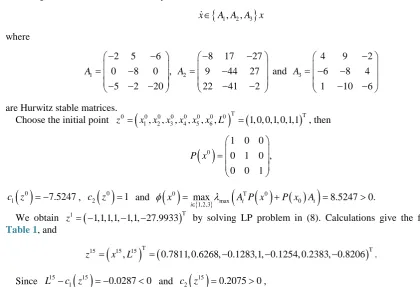
Example 1. Consider the switched system

{

1, 2, 3

}

x∈ A A A x

where

1 2 3

2 5 6 8 17 27 4 9 2

0 8 0 , 9 44 27 and 6 8 4

5 2 20 22 41 2 1 10 6

A A A

− − − − −

     

     

=_ − _ =_ − _ = −_ − _

₋ ₋ ₋   ₋ ₋   ₋ ₋ 

     

are Hurwitz stable matrices.

Choose the initial point z0 =

(

x x x x x x L₁0, ₂0, ₃0, ₄0, ₅0, ₆0, 0

)

T =

(

1, 0, 0,1, 0,1,1

)

T, then

( )

0

1 0 0

0 1 0 ,

0 0 1

P x

 

 

=  

 

 

( )

0

1 7.5247

c z = − , c2

( )

z0 =1 and

( )

_{ _}

(

( )

)

0 T 0

max 0

1,2,3

max i i 8.5247 0.

i

x A P x P x A

φ

λ

∈

= + = >

[image:4.595.81.502.425.712.2]

We obtain z1= −

(

1,1,1,1, 1,1, 27.9933− −

)

T by solving LP problem in (8). Calculations give the following

Table 1, and

(

)

T

(

)

_T

15 15 15

, 0.7811, 0.6268, 0.1283,1, 0.1254, 0.2383, 0.8206 .

z = x L = − − −

Since L15−c z1

( )

15 = −0.0287<0 and

( )

15

2 0.2075 0

(5)

Table 1. Kelley’s algorithm for Example 1.

k k

L 1

( )

k

c z 2

( )

k

c z

1 −27.9933 ‒209.7383 −1.9999

2 −24.4038 ‒127.1153 −2.3326

3 −14.2596 ‒106.2473 −1.8092

4 −10.0497 ‒63.4433 −1.8878

   

14 −0.8465 −1.1881 0.2694

15 −0.8206 −0.7919 0.2075

( )

15

0.7811 0.6268 0.1283

0.6268 1 0.1254

0.1283 0.1254 0.2383

P P x

−

 

 

= =_ − _

₋ ₋ 

 

is a common positive definite solution for

(

)

T

0 1, 2, 3 .

i i

A P+PA < i=

3. Stable Member in a Polytope

This part is devoted to the following question: Given a matrix family

{

A q

( )

:q∈B

}

where B⊂l is a compact, is there a stable matrix in this family?

In [12], a numerical algorithm has been proposed for a stable member in the affine matrix family

( )

{

A q :q∈l

}

. In this algorithm the uncertainty vector q varies in the whole space l. On the other hand we consider the case where q varies in a box B⊂Rl and use the gradient algorithm for minimization of the nonconvex maximum eigenvalue function. By choosing appropriate step-size, we obtain the convergence.

Let ₁, ₂, ,

(

1

)

2 r

n n Z Z Z _r= + _

 

 be a basis for the subspace of n n× symmetric matrices and

( ) ( )

(

T

( )

)

,

i i i i

Q q = −Z ⊕ A q Z +Z A q

( )

max

( )

1 ,

r

i i i

x q x Q q

φ λ

=

 

= _ _



∑



where x=

(

x x1, 2,,xr

)

T,

(

)

T 1, 2, , k

q= q q  q . Consider the problem

( )

T 1,

, minimize.

min 0

x q Q

x q

v P x v

φ

= ∈ →

>

Theorem 3. There is a stable matrix in the family A q

( )

if and only if φ* =min_{( )}_{x q}_, φ

( )

x q, <0.

Proof:

(

)

( )

* * * * *

1

0 there exists , such that 0

r

i i i

x q x Q q

φ

=

< ⇔

∑

<

( )

* T * * * *

0

r r r

i i i i i i

x Z A q x Z x Z A q 

     

⇔ −_ _⊕_ _− _{ }+ − _ _<

(6)

( )

_* _*

( ) ( ) ( ) ( )

_* T _* _* _* 1

0 and 0.

r

i i i

P x x Z A q P x P x A q

=

⇔ =

∑

> + <

By Lyapunov theorem, the matrix A q

( )

* is stable.

Example 2. Consider the family of matrices

( )

0 1 1 2 2 3 3, 1, 2, 3

[

1,1

]

A q =A +q A+q A +q A q q q ∈ −

where

0 1 2 3

1 0 2 0 2 0 3 0 1 0 2 0 1 0 0 1

2 0 3 0 1 0 3 2 3 1 3 0 1 2 3 2

, , , .

5 1 1 0 3 3 1 0 3 2 1 2 1 2 0 1

3 1 0 2 4 1 0 2 2 1 0 2 0 2 1 5

A A A A

− − −         ₋ ₋  ₋ ₋  ₋ ₋ ₋  ₋ ₋ ₋          = = = = − −  − −  − −   − −          − − − − − − − − − − −        

For q=

(

0, 0, 0

)

T, A q

( )

=A₀ is unstable. We apply the gradient algorithm to find a stable member in the family.

Let

T 0 1_{, 0, 0, 0, , 0, 0, , 0,}1 1 1

2 2 2 2

x =  _

  and

(

)

T 0

1, 0, 0

q = . So

(

)

T

0 0_, 0 1_{, 0, 0, 0, , 0, 0, , 0, ,1, 0, 0}1 1 1 _.

2 2 2 2

a = x q =  _

  Then

( )

( ) ( ) ( ) ( )

0 10 0 0 T

0 0 0 0

1

0

1 2 0 0 0 0 0 0 0

0 1 2 0 0 0 0 0 0

0 0 1 2 0 0 0 0 0

0 0 0 1 2 0 0 0 0

.

0 0 0 0 1 0 5 0

0 0 0 0 3 0 6 2

0 0 0 0 8 4 2 0

0 0 0 0 7 2 0 4

i i i

P x x Q q

A q P x P x A q

= ₋    = _ ₊ _   −    ₋     −    −   =  ₋    − −    ₋ ₋     ₋ ₋ ₋   

∑

Maximum eigenvalue of this matrix and its corresponding unit eigenvector are

(

)

T

max 2.1866,v 0, 0, 0, 0, 0.7644, 0.4480, 0.1668, 0.4324

λ

= = − − −

respectively. Gradient of the function φ at a0 is

(

)

0

T

2.44, 1.86, 11.04, 2.78,1.93, 7.50, 4.30, 2.52, 7.46, 2.35, 0.28, 0.50, 2.73 . a

φ

∇ = − − − − −

The first tencomponent of the vector 0

1 0

a

a =a − ⋅∇t

φ

should be on the ten dimensional unit sphere. There-fore t=0.01531 and

(

)

T

1

0.53, 0.02, 0.16, 0.04, 0.47, 0.11, 0.06, 0.46, 0.11, 0.46, 0.99, 0.007, 0.04 .

a = − − − −

After 4 steps, we get

(

)

(

)

T

4 4 4

, 0.59, 0.03, 0.04, 0.009, 0.41, 0.05, 0.04, 0.49, 0.15, 0.45, 0.98, 0.03, 0.08

(7)

and

φ

(

x q4, 4

)

= −0.2585<0. Therefore A q

( )

4 is stable.

4. Conclusion

Two important problems from control theory are considered: the existence of common quadratic Lyapunov functions for switched linear systems and the existence of a stable member in a matrix polytope. We obtain new conditions which give new effective computational algorithms.

References

[1] Boyd, S. and Yang, Q. (1989) Structured and Simultaneous Lyapunov Functions for System Stability Problems. Inter-national Journal of Control, 49, 2215-2240. http://dx.doi.org/10.1080/00207178908559769

[2] Büyükköroğlu, T., Esen, Ö. and Dzhafarov, V. (2011) Common Lyapunov Functions for Some Special Classes of Sta-ble Systems. IEEE Transactions on Automatic Control, 56, 1963-1967. http://dx.doi.org/10.1109/tac.2011.2137510

[3] Cheng, D., Guo, L. and Huang, J. (2003) On Quadratic Lyapunov Functions. IEEE Transactions on Automatic Control,

48, 885-890. http://dx.doi.org/10.1109/tac.2003.811274

[4] Dayawansa, W.P. and Martin, C.F. (1999) A Converse Lyapunov Theorem for a Class of Dynamical Systems Which Undergo Switching. IEEE Transactions on Automatic Control, 44, 751-760. http://dx.doi.org/10.1109/9.754812

[5] King, C. and Shorten, R. (2004) A Singularity Test for the Existence of Common Quadratic Lyapunov Functions for Pairs of Stable LTI Systems. Proceedings of the American Control Conference, Boston, 30 June-2 July 2004, 3881- 3884.

[6] Mason, O. and Shorten, R. (2006) On the Simultaneous Diagonal Stability of a Pair of Positive Linear Systems. Linear Algebra and Its Applications, 413, 13-23. http://dx.doi.org/10.1016/j.laa.2005.07.019

[7] Narendra, K.S. and Balakrishnan, J. (1994) A Common Lyapunov Function for Stable LTI Systems with Commuting A-Matrices. IEEE Transactions on Automatic Control, 39, 2469-2471. http://dx.doi.org/10.1109/9.362846

[8] Shorten, R.N. and Narendra, K.S. (2002) Necessary and Sufficient Conditions for the Existence of a Common Qua-dratic Lyapunov Function for a Finite Number of Stable Second Order Linear Time-Invariant Systems. International Journal of Adaptive Control and Signal Processing, 16, 709-728. http://dx.doi.org/10.1002/acs.719

[9] Shorten, R.N., Mason, O., Cairbre, F.O. and Curran, P. (2004) A Unifying Framework for the SISO Circle Criterion and Other Quadratic Stability Criteria. International Journal of Control, 77, 1-8.

http://dx.doi.org/10.1080/00207170310001633321

[10] Liberzon, D. and Tempo, R. (2004) Common Lyapunov Functions and Gradient Algorithms. IEEE Transactions on Automatic Control, 49, 990-994. http://dx.doi.org/10.1109/tac.2004.829632

[11] Polyak, B.T. and Shcherbakov, P.S. (2005) Hard Problems in Linear Control Theory: Possible Approaches to Solution. Automation and Remote Control, 66, 681-718. http://dx.doi.org/10.1007/s10513-005-0115-0

[12] Polyak, B.T. and Shcherbakov, P.S. (1999) Numerical Search of Stable or Unstable Element in Matrix or Polynomial Families: A Unified Approach to Robustness Analysis and Stabilization. Robustness in Identification and Control Lecture Notes in Control and Information Sciences, 245, 344-358. http://dx.doi.org/10.1007/bfb0109879

(8)