The London School of Economics and Political Science
Predictability and the decay of
information in mathematical and physical
systems
Ewelina Sienkiewicz
A thesis submitted to the Department of Statistics
of the London School of Economics for the degree of Doctor of Philosophy.
Declaration
I certify that the thesis I have presented for examination for the MPhil/PhD degree of the London School of Economics and Political Science is solely my own work other than where I have clearly indicated that it is the work of others (in which case the extent of any work carried out jointly by me and any other person is clearly identified in it).
The copyright of this thesis rests with the author. Quotation from it is permitted, provided that full acknowledgement is made. This thesis may not be reproduced without my prior written consent.
I warrant that this authorisation does not, to the best of my belief, infringe the rights of any third party.
I declare that my thesis consists of less than 100,000 words.
Statement of conjoint work
I confirm that chapter 7 was jointly co-authored with Dr Erica L Thompson and I contributed to 95% of this work.
Abstract
This thesis explores the predictability of nonlinear systems, both mathematical sys-tems (as realised on a digital computer) and geophysical syssys-tems (the El Ni˜no Phe-nomena, and climate prediction via downscaling). How far into the future does a forecast system provide information beyond that available purely from the past? How does information in a probabilistic forecast decay with time? Is it true that, no matter how good the simulation model used for prediction is, there will be a point where predictability is lost? That is, that there is always a time horizon beyond which any forecast fails to yield useful information.
The two main limits to predictability are identified and discussed. Sensitivity to initial condition complicates the forecasting of chaotic dynamical systems, even when the model is perfect. Structural model error (model inadequacy) is a distinct cause of the decay of predictability, a decay that may often be mistakenly interpreted as resulting from chaos. These features are distinguished and demonstrated both in low-dimensional mathematical systems and weather and climate models.
Model inadequacy is shown to be important in real-world forecasting, with ref-erence to Columbia University's C-Z model for El Ni˜no predictions and climate models used in the North American Regional Climate Change Assessment Program (NARCCAP). Repercussions for forecast performance are discussed. In short, (i) NARCCAP regional simulations are quickly inconsistent with the global simula-tions used to drive them, (ii) the C-Z model allows experiments into the decay of predictability when one model version is employed as the system, and a second, structurally distinct model version is used as the model.
The decay of predictability is studied from the view point of information theory. Information theoretic tools are allied both to mathematical system-model pairs and to physical system-model pairs. A flaw in formulating one such tool, proposed by Du and Smith (2012, PRE) is exposed and alternative normalisations are explored in various experiments. A quantity called the information deficit, introduced in that same paper, is considered in several settings. New properties of the information deficit are discovered, and it is demonstrated that the information deficit can be a useful tool in identifying (and correcting) shortcomings of a forecasting system.
Acknowledgements
I would like to express my gratitude to all the wonderful people mentioned here. They supported me in my research over the last few years and helped me bring the PhD thesis to the finish line.
To my supervisor Professor Leonard Smith, thank you for giving me directions and guidance and for sharing your unlimited enthusiasm and wisdom. You made my PhD studies exciting and inspiring.
To Dr Erica Thompson and Dr Edward Wheatcroft, it has been a pleasure working with you. Thank you for all your greatly appreciated help and advice and for being so generous with your time.
To my husband Konrad for being supportive, positive and fulfilling a huge list of day-to-day duties exceedingly well.
Finally, to my mother and little daughter Nell for bringing lots of love and joy to every day.
Contents
1 Introduction 1
2 Introduction to Predictability of Dynamical Systems 7
2.1 Nonlinear dynamical systems . . . 8
2.2 Climatology . . . 10
2.3 Chaos . . . 11
2.4 System-Model pair . . . 11
2.5 Perfect and Imperfect Model Scenarios . . . 12
2.5.1 Perfect Model Scenario . . . 12
2.5.2 Imperfect Model Scenario . . . 12
2.6 Ensemble forecasting . . . 13
2.7 Summary . . . 14
3 Tools for Measuring Predictability 15 3.1 Predictability . . . 16
3.1.1 The decay of predictability . . . 17
3.1.2 Limitations to predictability . . . 17
CONTENTS v
3.2 Skill Scores . . . 18
3.3 Ignorance . . . 19
3.3.1 Climatological Ignorance . . . 20
3.3.2 Empirical Ignorance . . . 21
3.3.3 Model Implied Ignorance . . . 21
3.3.4 Alternative normalisation . . . 22
3.4 Information Deficit . . . 23
3.5 Relative Entropy . . . 25
3.6 From Ensembles to Probability Forecasts . . . 27
3.6.1 Kernel density estimation . . . 28
3.6.2 Kernel dressing . . . 28
3.6.3 Blending with climatology . . . 29
3.6.4 Model selection techniques . . . 30
3.6.5 Cross-validation . . . 31
3.7 Conclusions . . . 31
4 Distinguishing model inadequacy from chaos in nonlinear simula-tion 33 4.1 Illustration with Henon Map: single and double precision . . . 34
4.1.1 Divergence of specific Initial Conditions . . . 34
4.1.2 Divergence averaged over the attractor . . . 39
4.2 Illustration with Henon Map and Senon Map . . . 41
4.2.1 Experimental design . . . 41
CONTENTS vi
4.2.3 How does this relate to a weather-like climate-like context? . . 47
4.3 Illustration with Ikeda Map . . . 47
4.4 Conclusions . . . 50
5 The Decay of Predictability 51 5.1 Logistic and Quartic Maps . . . 52
5.1.1 Model and System . . . 52
5.1.2 Relative Entropy (RE) between the model and the system . . 56
5.1.3 Bifurcation Diagram of the model and different versions of the system . . . 59
5.2 Demonstrating the decay of information . . . 62
5.2.1 Ensembles and Climatology . . . 62
5.2.2 Operational parameters for use in forecasting . . . 64
5.2.3 Decay of Information . . . 66
5.2.4 Shortcomings of normalisation method D . . . 77
5.3 Logistic Map as a model for alternative systems . . . 78
5.4 Conclusions . . . 86
6 Modelling the real world: Predictability in probabilistic modelling of El Ni˜no 88 6.1 El Ni˜no . . . 89
6.1.1 What is El Ni˜no? . . . 89
6.1.2 El Ni˜no in the Pacific . . . 93
6.1.3 El Ni˜no and the World . . . 95
CONTENTS vii
6.2 Cane-Zebiak model . . . 98
6.2.1 Information about the model . . . 98
6.2.2 Qualitative Behaviour . . . 100
6.3 Decay of information in the Cane-Zebiak model - Perfect Model Scenario104 6.3.1 Generation of ensemble-based probabilistic forecasts of the NINO34 Index . . . 104
6.3.2 Climatology for NINO34 for the C-Z model . . . 108
6.3.3 Adjusting parameters of kernel dressing of Ni˜no 3.4 Index en-semble forecasts . . . 121
6.3.4 Predictability measures applied to the Perfect Model . . . 128
6.4 Predictablity and Forecasting given an Imperfect Model . . . 140
6.5 Effect of not having a representative climatology . . . 145
6.6 Conclusions . . . 147
7 Dynamical downscaling of climate model projections: consequences for predictability 149 7.1 Introduction: Aims of dynamical downscaling of climate simulations . 150 7.2 The NARCCAP downscaling project . . . 151
7.3 NARCCAP data and definitions of study regions . . . 153
7.3.1 RCM/GCM pairs used . . . 153
7.3.2 Definition of study areas . . . 155
7.4.3 Comparison of short- and medium-term average precipitation
(joint work with Dr Erica Thompson, LSE) . . . 164
7.5 Does RCM improve GCM output towards the real-world? . . . 166
7.6 Conclusions . . . 169
8 Conclusions 172 Nomenclature 174 Appendix A System-Model pairs used in Chapter 4 177 A.1 Henon Map . . . 177
A.2 Senon Map . . . 178
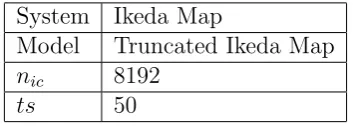
A.3 Ikeda Map . . . 179
A.4 Truncated Ikeda Map . . . 180
Appendix B Climatology of the Quartic Map 182 Appendix C Details of Imperfect Model of C-Z model 187 C.1 Comparison with the 10-day model . . . 188
C.2 Additional analysis for section 6.4. . . 189
Bibliography 189
List of Tables
4.1 Experimental Design 4.A . . . 42
4.2 Experimental Design 4.B . . . 48
5.1 These three maps will be repeatedly used in the chapter: Pure Lo-gistic, Full Quartic and the map that mixes both together, which is called Quartic. . . 53
5.2 Experimental Design 5.A . . . 53
5.3 Experimental Design 5.B . . . 56
5.4 Experimental Design 5.C . . . 59
5.5 Experimental Design 5.D . . . 63
5.6 Experimental Design 5.E . . . 79
6.1 Experimental Design 6.A . . . 105
6.2 Experimental Design 6.B . . . 107
6.3 Experimental Design 6.C . . . 110
6.4 Experimental Design 6.D . . . 115
6.5 Relative Entropy by size of the sample (nic ) and number of bins
(k) for equally likely bins case in experiment 6.D. Data was drawn from the uniform distribution 220 times, values in the table show RE
averaged over the number of repetitions. The bigger the number of bins (k) the bigger theRE. It decreases proportionally to the increase in the size of the sample (nic ). . . 116
6.6 Relative Entropy by size of the sample (nic) and number of bins (k)
for unequally likely bins case in experiment 6.D. Data was drawn from the uniform distribution 220 times, values in the table show RE
averaged over the number of repetitions. Here conclusions are the same as in Tab.6.5. The bigger the number of bins (k) the bigger the RE. It decreases proportionally to the increase in the size of the sample (nic ). . . 116
6.7 Difference in Relative Entropy by size of the sample (nic) and number
of bins (k) between 2 methods: equally and unequally likely bins in experiment 6.D. Data was drawn from the uniform distribution 220
times, values in the table show RE averaged over the number of repetitions. There is not much of a difference between the methods. In most of the cases RE for unequally likely bins is bigger. . . 117 6.8 Operational parameters and Ignorance in October in year 24 derived
from the in-sample and out-of-sample sets in experiment 6.B. As ex-pected, minimum Ignorance and blending parameters between sets are different. These results are the coordinates of the red dot in Fig-ure 6.15 (a) and (b). . . 123 6.9 Experimental Design 6.E . . . 141
List of Figures
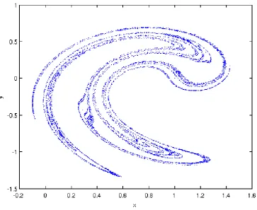
2.1 The Ikeda attractor as defined in Appendix A.3. In the long term, all initial conditions will converge to this attractor. . . 9
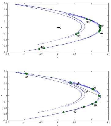
4.1 The two panels show two trajectories with slightly different initial con-ditions iterated under the same dynamics. The separation between these initial conditions is ε = (2−10, 2−10). After 32 to 40 iterations the trajectories look very different. The distance between a pair of points (black line), depends on the location of the initial condition. For example distance at lead time 40 is bigger in the bottom chart than in the top one. . . 36 4.2 The same Initial Condition (IC) was evolved under two different
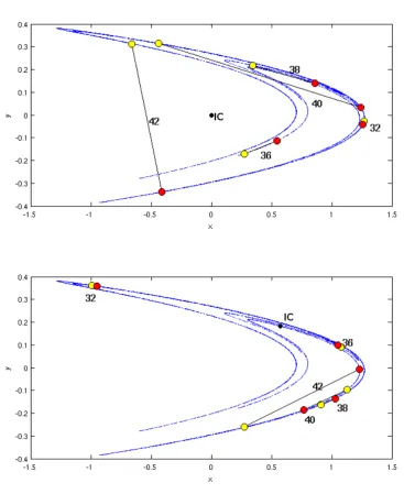
dy-namics: single (yellow) or double (red) precision Henon Maps. Some-where between 32 and 40 iterations later both trajectories originating from the same initial condition are far apart. The distance between points (black line), depends on where on the chaotic system the initial condition is built. . . 38
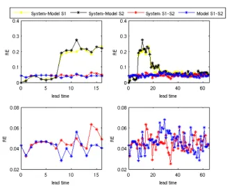
LIST OF FIGURES xii 4.3 Mean Euclidean distance between trajectories originating from many
distinctly located initial conditions of a pair of points as a function of lead time in a situation of model inadequacy (top left) and chaos (top right) as illustrated in Figs.4.1 and 4.2. Bars along the green and the red curves represent 95% re-sampling intervals of the mean. As shown in the top charts, the divergence of the trajectories increases with time in a different way. The bottom chart illustrates the difference between the two charts at the top. These results demonstrate that model inadequacy and chaos are two different sources of forecast failures and should be distinguished when considering future resource allocation. . 40 4.4 Processes in Experiment 4.A. . . 42 4.5 Sets of points ‘1’ (yellow) and ‘2’ (black) within a Gaussian ball for
each standard deviation (Sd). Note the charts have different scales
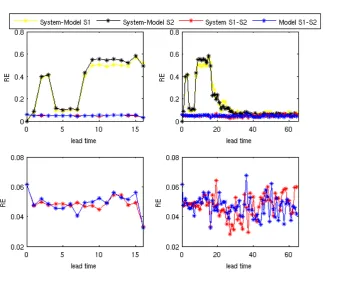
on their X and Y axes. . . 43 4.6 RE as a function of lead time for the first 16 time steps (left panel)
and 64 time steps (right panel) in Experiment 4.A, forSd= 0.01. The
yellow and black lines show how one set of initial conditions behave differently under the different dynamics of the system and the model. TheRE of S1 and S2 developed using the dynamics of the system or model is illustrated with red or blue lines respectively. . . 45 4.7 This figure is the same as Fig.4.6, but concerns smaller noise level
(Sd = 0.001). . . 46
LIST OF FIGURES xiii 5.1 The minimum (blue), maximum (red) and the mean (black)
propor-tion of points falling into each bin over 4 sets of draws for a) µ = 0 and b) µ = 1 under the experiment 5.A. Both distributions have greater probability nearx=0 andx=1. However the distributions are not the same. For example, there is a contrast between the min, mean and max in the first bin at the lower edge of the range ofx. . . 55 5.2 The RE between the model and the system for different values of
µ in experiment 5.B. Note the different scale between chart (a) and (b). Each solid line corresponds to a different model run. TheRE is largest when µ = 1, which is when when the system is fully quartic. Forµ∈(2−4,20)RE increases quickly, for ≤ 2−4 it stays in a similar
range. The dashed lines show the range of RE between model and itself for different model realisations. For µ > 2−4 there is clear evi-dence that the distributions of the model and the system are different. 58 5.3 Bifurcation Diagrams for experiment 5.C, where a) µ= 0 (shown in
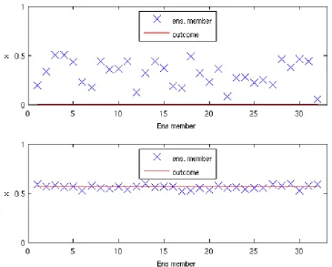
green), b)µ= 0.1 and c)µ= 1 (system is Full Quartic). Qualitative behaviour did not change between diagrams a) and b). Diagram c) shows different behaviour. For example, with µ = 1 the period doubling cascade is complete beforer=3.5. Also, the period-3 window (near r=3.83) shifts left from a) to c). . . 61 5.4 An example of initial condition ensemble for the experiment 5.D. The
chart illustrates the location of 32 ensemble members. Each blue star represents an ensemble member, while the red line represents the outcome. All ensemble members will correspond to the same outcome. 64 5.5 Operational kernel dressing parameters as a function of lead time in
experiment 5.D2. The red line shows the kernel width σ and the
black line shows the blending parameter α. For short lead times, α
LIST OF FIGURES xiv 5.6 Climatological Ignorance using each method as a function of lead
time. Method D (mD) assumes that target forecasts are random draws from the climatology. Method E (mE) is the Mean Ignorance when using climatology as a forecast. Values of the Climatological Ignorance calculated in methods D and E are in a similar range, but are not exactly the same. . . 68 5.7 Mean Ignorance as a function of lead time for two methodologies (mD
and mE), in experiment 5.D. It increases in the first 8 time steps and for method E at the 9th lead time converges to 0. When the Empirical Ignorance is zero, the forecast is equal to the climatology so it is not useful. There is no big difference between mD (left panel) and mE (right panel). Here we note that method D is positive at time step 8, though the resampling interval includes 0. . . 69 5.8 Empirical Ignorance calculated using two methodologies (mD and
mE) for experiment 5.D. Each thin line shows the Ignorance of a different ensemble forecast, whilst the thick line shows the Empirical Ignorance. Climatological Ignorance in mE brings all forecasts to zero from time step 9 while in mD they do not converge. At initial time steps, the Ignorance is often much greater than zero in both methods. This is expected and explained in Fig.5.9. . . 70 5.9 Examples of ensembles (blue crosses) and the outcomes (red lines) for
a case in which the outcome falls outside of the range of the ensemble (top) and within the range of the ensemble (bottom). The ensemble at the top will tend to result in a positive ignorance score (see Fig.5.8). 71 5.10 Model Implied Ignorance as a function of lead time for method mD
(left) and mE (right) in experiment 5.D. Whilst method E always stays non-positive, this is not the case for method D. . . 72 5.11 Components that are subtracted (see equations 3.6 and 3.9) when
LIST OF FIGURES xv 5.12 Model Implied Ignorance calculated using two methodologies (mD
and mE), for experiment 5.D. Each thin line shows the Model Im-plied Ignorance for a different ensemble, whilst the thick lines show the mean over all forecasts at each lead time. In both methods, fore-casts converge to zero from time step 9, since α = 0. In mD the Climatological Ignorance takes the Model Implied Ignorance above zero in some cases. . . 74 5.13 Empirical Ignorance (solid line), the Model Implied Ignorance (dashed
line) and the Information Deficit (black line) as a function of lead time for methods D (left) and E (right). Whilst the Information Deficit is non-negative for method E, this is not the case for method D. . . 76 5.14 Information Deficit calculated using method D (left) and E (right)
with 95% resampling intervals as a function of lead time. For method D, there is significant evidence that the Information Deficit is negative in 4 lead times. . . 77 5.15 The Information Deficit as a function of lead time for different values
of µ. The Information Deficit is positive and larger, in general, for the highest level of model imperfection. The larger theµ, the quicker the Information Deficit reaches zero. This is because the blending parameter α decays to zero quicker. The dashed line shows the In-formation Deficit when µ = 0.5 and the model is not blended with climatology. The Information Deficit tends to be the largest in this case and never reaches 0. . . 81 5.16 Empirical Ignorance (solid line) and the Model Implied Ignorance
LIST OF FIGURES xvi 5.17 Empirical Ignorance when µ=0.01 and 0.5. Each thin line represents
a different forecast. The black thick curve shows the Mean Ignorance over all forecasts with the error bars representing 95% resampling in-tervals of the mean. For longer lead times, the Ignorance converges to 0. There are some bad forecasts (those with the Empirical Ignorance well above 0) at the beginning of the simulation for each of these two cases of µ. The score forecast is much worse for µ=0.01 than 0.5, with the Empirical Ignorance being greater than 10 (see chart on the left). This happens when, for example, ensemble members are far from the target forecast and the kernel width is too small to capture them (see Fig.5.9). If operational parameters used to calculate the forecast are modified as discussed in the text, the number of ‘bad’ forecasts decreases (see Fig.5.18). . . 84 5.18 Empirical Ignorance by time step forµ=0.01 calculated with modified
α and σ. This should be compared with the left panel of Fig.5.17. Doubling of the kernel widthσ or decreasingαby one eighth for each time step reduced the number of ‘bad’ ensemble forecasts. . . 85
6.1 Graphical illustration of the four Ni˜no regions in the tropical Pacific, by NOAA Climate Prediction Center [7]. These are the regions used by the C-Z model. . . 90 6.2 3-month average sea surface temperature (SST) anomalies in the Ni˜no
3.4 region. The figure illustrates irregularity in the length and occur-rence of the events since 1950. The latest warm phase in 2015-16 was very strong with the anomaly above the 2◦C threshold. (Courtesy of NOAA [7]). . . 92 6.3 Fig. a) shows average ocean temperature in the Pacific between
LIST OF FIGURES xvii 6.4 Map in the left panel illustrates total rainfall in Jan-Mar 1998, during
a very strong El Ni˜no. The heaviest rainfall at that time is shown by the darker green and blue colours. Analogically to Fig.6.3 the map on the right shows departures (x100)mm from the average. The dark green in the right picture indicates 400 mm more than average, so the rainfall was double the average in this region. By contrast, the dark grey region of Indonesia has, on average, 800 mm and in Jan-Mar 1998 had no precipitation at all, resulting in extreme dryness. (Courtesy of NOAA [7]). . . 94 6.5 Effects of El Ni˜no on global climate in winter (top) and summer
(bottom) by NOAA [7]. Whilst these effects are more likely in El Ni˜no years, they are not guaranteed. . . 96 6.6 Examples of time series of the monthly NINO34 index for 64 years
from the C-Z model (red and blue lines) vs. 1950-2014 observations by NOAA (black dotted line)[7]. Initial conditions in the top and the bottom charts are different. In both cases we observe aperiodic cycles of warm phases with an average occurrence period of 4 years. The range of the index is between -2 and 3◦C. The model appears to illus-trate fluctuations in SST in the tropical Pacific reliably (see section 6.1.1 for more details). This behaviour is similar to observations, and the model looks non-linear. . . 101 6.7 Trajectories of the 10-day model (used in the Perfect Model Scenario)
LIST OF FIGURES xviii 6.8 Trajectories of the NINO34 index of the C-Z model with 3 different
noise levels. Nearby initial conditions separate from the target fore-cast. At year 10 we observe that the time series representing the smallest noise level of 1/128 (red dotted line) stays the closest to the outcome (green solid line). The biggest noise level of 1/32 (blue dotted line) is the furthest from the target forecast. . . 103 6.9 Example of an ensemble forecast of the NINO34 index evolved on
the C-Z model in experiment 6.B. There are 64 scenarios shown with black lines. The green line is the outcome. Most members stay close to the target forecast for the first 2 years, that is when the forecast is good. Then at year 3, if we turned nearby initial conditions into a probability forecast it would be a bimodal pdf, because members of the ensemble oscillate around two values. At year 3.5 there is a return to a skill, when everything is back in the same place again. At years 4 and 5 we have something bimodal, in year 5.5 all mem-bers are together again and we have a good forecast. Then nearby initial conditions get separated along the attractor. This behaviour would not be the same for every ensemble. This example illustrates a sensitivity to initial condition. . . 108 6.10 Relative Entropy (RE) between two distributions of Clim1 and Clim2
in experiment 6.C. This is plotted for 64 years in May for (a -top chart) a case with equally likely and (b -bottom chart) equally spaced bins. On a scale of 50 years RE approaches the sampling error line, which means that probability distributions representing both methods look similar after that time. We notice here, that the shape of the
LIST OF FIGURES xix 6.11 Proportion of 2048 Gaussian perturbations around 1 IC (Clim2)
rela-tive to a Clim1 in time and by bin, experiment 6.C. In fig.(a) equally likely, in (b) equally spaced bins are shown. Colour relates to the pro-portion of model elements in that box. Black means the most likely, light yellow indicates the least probable. Each vertical slice adds up to one. At the beginning all elements are in the same box. Here we start with all light yellow and one black box, which becomes lighter with a time. Colour in boxes flickers with a time step. In case (a) with equally probable bins, each box is the same at the end, because all elements are equally spread around each bin. In case (b), box 4 is the most likely after 60 years. Fig.(a) decays flat and fig (b) decays to climatology. Gaussian perturbations spread around all bins quicker in case (a) than (b). There are still oscillations in almost every box (see orange stripes across every bin), which suggests that the information has not been lost. . . 114 6.12 Tail of the RE curve shown in Fig.6.10. Here RE is above the
sam-pling error (calculated in Tables 6.5 or 6.6) with 95% resamsam-pling intervals for both (a) equally likely and (b) equally spaced bins. This could mean that the data used in the experiment 6.C is too short for the model to converge to the system, and could explain the pattern across bins (orange stripes) in Fig.6.11, still visible after 60 years. . . 118 6.13 Climatology of NINO34 index for C-Z model (solid line) and
1950-2016 observations by NOAA (dotted line). Shapes of probability den-sity estimate between (a) August and (b) December are very different. In case (a) the model is around one state - 0◦C, while in case (b) it is spread around different possibilities. This corresponds to the ob-servations, as the NINO34 index reaches its extremes in winter and diminishes in summer. In case (b) the model does not capture the entire range of values. . . 120 6.14 Operational kernel dressing parameters: the kernel widthσ (red line)
LIST OF FIGURES xx 6.15 Ignorance by weight (α) and kernel width (σ) at year 24 in Oct.
The mean ignorance of the in-sample set (top) and out-of-sample set (bottom) at year 24 in October, as a function of α and σ. The red dot shows the point at which the mean ignorance is minimised in each case. The black line shows the lowest value on this surface. This demonstrates how the optimised parameters can be sensitive to the sample used. . . 124 6.16 Contour plot of mean Ignorance with α and σ. The Mean Ignorance
tends to decrease when α increases and σ decreases. Here, we also notice that as we move to bigger α, the optimal value of σ tends to increase. The red dot shows combination of α and σ that minimises the mean Ignorance as shown in Fig.6.15. . . 125 6.17 Relative entropy between the forecast and the climatology for May
as a function of lead time for equally likely (top) and equally spaced (bottom) bins for the in-sample (red) and out-of-sample (blue) sets. After around 40 years, the forecasts and the climatology are very sim-ilar and thus the RE is close to zero and around the sampling error (calculated in Tables 6.5 or 6.6). As expected, the RE is smaller in case (a) than (b) in the first years of the simulation, because fluctua-tions are smaller. In case (b) when bins are equally spaced, variation of bins with fewer members is big, so the RE is big for those bins.
RE of in-sample set vs. climatological distribution (blue line) is not the same as out-of-sample set vs. climatology (red line), as both sets are different. . . 127 6.18 In-sample vs. out-of-sample Empirical Ignorance. Markers show
con-secutive years of May and stay near diagonal. This means in-sample and out-of-sample sets are similar and the derived operational param-eters are robust. . . 128 6.19 Empirical Ignorance as a function of year for Jan, Apr, Jul and Oct
LIST OF FIGURES xxi 6.20 Empirical Ignorance for each individual forecast for the month of
October in experiment 6.B. Each thin line shows the Ignorance of a different ensemble forecast, whilst the thick black line shows the mean Ignorance over all forecasts. Some forecasts have Ignorance greater than zero for long lead times. This is expected and explained in the top chart of Fig.6.21. . . 131 6.21 Top panel: example of ensemble probability density (blue line) and
the outcome (red cross) for a case in which the outcome falls outside of the range of the ensemble. The ensemble at the top, resulted in a positive Ignorance score (see red line at year 25 in Fig.6.20). The bottom chart shows the outcome (blue cross) which falls outside the range of climatology. This resulted in a large Climatological Igno-rance, which made the Empirical Ignorance very low (see yellowish line at year 52 in Fig.6.20.) . . . 132 6.22 Model Implied Ignorance as a function of lead time for four months of
the year in experiment 6.B. The Model Implied Ignorance is negative for shorter lead times but tends to zero as our forecasts approach the clmatology. This pattern is similar to the example shown using the simple mathematical model in the previous chapter (Fig.5.10, for example). In contrast to that example however the Model Implied Ignorance does not grow monotonically, but jumps up and down. This issue is explained in Fig.6.24. . . 134 6.23 Model Implied Ignorance as a function of lead time for the month
LIST OF FIGURES xxii 6.24 Climatology in November (blue bars) and Ensemble forecast A
(pur-ple dots) in November at year 1 and at year 2. Ensemble forecast A falls into a range of climatology which puts high probability (top) and low probability (bottom). The ensemble at the bottom resulted in a drop of the Model Implied Ignorance by 6 bits from year 1 to year 2. . . 136 6.25 Information Deficit in Jan, Apr, Jul and Oct. The Information Deficit
is non-negative, as the 95% resampling intervals include 0. In general, the Information Deficit is small, it decreases with years and stays around 0 for longer lead times. If we had data for another 64 years, we would expect that the Information Deficit would converge to 0, as it does in the mathematical model case (see green line in Fig.5.15). . 139 6.26 Operational parameters for the months of Jan, Apr, Jul and Oct as a
function of lead time for the imperfect model case in experiment 6.E. The red line shows kernel width σ and the black line the weight α. Hereα decays faster than in the perfect model case (see Fig.6.14). . . 142 6.27 Information Deficit for January, April, July and October, Imperfect
LIST OF FIGURES xxiii 6.28 Minimum and Maximum value of NINO34 by month for
climatolog-ical set against (from the left): min/max of outcomes, min/max of ensemble forecasts (from PM) and min/max of ensemble forecasts (from IM). If the climatology was good, we would see in the graphs that red stars are above red diamonds and blue stars are below blue diamonds. However, we observe a different pattern. Climatologi-cal range is often not covering the range of outcomes or ensembles. This could result in a large value of Climatological Ignorances and requires additional assumptions while computing the Model Implied Ignorance. Transient states contribute to this difference. . . 146
7.1 Maps showing the study areas as a grid on RCM. In this research we refer to them as (from the top) USA area, South-East and North-West of the USA. . . 156 7.2 Maps illustrate difference in long-term averages (over 1991-2000) of
surface radiation upward (variable ‘rlus’) between RCM output and its driving data by the grid point. The results concern the following NARCCAP RCM-GCM pairings: a) ECP2-gfdl, b) CRCM-ccsm, c) CRCM-cgcm3, d) MM5I-ccsm, e) WRFG-cgcm3. The average differ-ence for the USA area is: -8 W/m2; -3 W/m2; -4 W/m2; -16 W/m2
LIST OF FIGURES xxiv 7.3 Each point in this diagram represents a single monthly average, is
coloured by the interval of simulation it falls into (beginning: 1968-1980 -black, middle: 1981-1990 -blue, end: 1991-2000 -red), and its shape depends on the month name. X axis shows RCM surface radi-ation upward value, Y axis shows RCM/GCM ratio. Charts concern the following regions: US area, North West, South East. Data Source: ECP2-gfdl, NARCCAP. Most points lie below the line of equality be-cause radiation in the RCM is generally lower than in its parent GCM. Results at regional level are, as expected, more varied than at country level, but even over the whole US area, there is a 2-5 % discrepancy in January, April and July on absolute values which are greater than 400 W/m2, so an absolute discrepancy of over 8 W/m2. Summer months show the biggest difference in the radiation. For July time series see Fig.7.4. . . 162 7.4 July averages of surface radiation upward over 1968-2000 by region
and model type. Data Source: ECP2-gfdl, NARCCAP. Note the difference of 50-60 W/m2 between GCM and RCM in SE. At the
country level radiation is on average 10 W/m2 lower in the RCM
than the parent GCM. . . 163 7.5 Difference between RCM and GCM for precipitation over the
NARC-CAP study area, for a single month (January 1991), averaged over 5 years (1991-5), and monthly averages over the whole study area. This figure was generated by Dr Erica Thompson of LSE and is gratefully used with her permission [108]. . . 165 7.6 Charts illustrate annual averages between 1991-2000 of surface
LIST OF FIGURES xxv 7.7 Matching an observation point with RCM, and GCM grids. Here,
Austin Camp Mabry Texas, US (black rectangle) and the correspond-ing grid centres on the RCM (yellow circle) and GCM (dark green triangle). RCM grid is illustrated by grey circles, GCM grid by blue triangles. Note that the centre of RCM or GCM grid do not cover the coordinates of the studied location. The best match is the near-est point on the grid of the model from longitude and latitude of the place of interest. . . 168
A.1 Attractor of (a) classical Henon Map and (b) Senon Map [93] with parameters as described above. These attractors look very similar, but yield different results as described in experiment 4.A. on distin-guishing model inadequacy and chaos. . . 179 A.2 Attractor of Ikeda Map (top chart) and Truncated Ikeda Map (bottom
chart) with parameters as described above. . . 181
B.1 Sample climatology when µ=0 and µ=0.5. There is a noticeable dif-ference between probability density for both climatologies at the edges of x. . . 183 B.2 Sample climatology when µ=0 vs. beta distribution with a=0.5 and
b=0.5. Colour of crosses show different runs of the sample climatol-ogy. The difference between runs is hard to distinguish. Stars show probability density by beta function for x=0.01:0.01:0.99. Sample climatology is in line with beta function (red curve). As expected, crosses which show probability density at the edges of each bin, are on the beta function curve, in the middle between red stars. . . 184 B.3 Probability density estimate of climatology derived by evolving set of
C.1 Example of an ensemble forecast as a function of time for the 10-day model (top chart) and the 5-day model (bottom chart), experiment 6.E. Ensembles spread around different values of NINO34 index at different paces - quicker for the 10-day model and at different ranges - wider for the 10-day model. . . 188 C.2 An ensemble forecast shown as a function of time in the Imperfect
Model scenario over 64 years in May along with outcome for each year. Each line shows a member of the ensemble while a black star illustrates the outcome in each year. In some years, the ensemble is far from the outcome, which results in the Empirical Ignorance being positive. . . 189
Chapter 1
Introduction
The main theme of this thesis is predictability and the exploration of useful informa-tion in nonlinear forecasting situainforma-tions. Two distinct factors that limit predictability of nonlinear models, specifically structural model error and uncertainty in the ini-tial condition, are explored in various experiments. We consider predictability from the perspective of information theory. Throughout the thesis, models are used to form probabilistic forecast distributions and information is quantified in terms of information (measured in bits) with reference to some baseline. Climatology, which comprises of typical values derived from a large number of past observations of the system, serves as this reference standard.
This chapter provides an overview of the thesis. Some terminologies may be new to the reader and are explained in later chapters when they are used for the first time. In short, the thesis is structured as follows: chapter 2 and chapter 3 pro-vide background knowledge used and explored throughout the thesis. Broadly, the mathematical content can be found in chapter 4 and 5, while applications to two
2
real-world modelling systems are described in chapter 6 (the Cane-Zebiak [21] model of El Ni˜no) and chapter 7 (the set of NARCCAP models of the Earths climate, fo-cused on North America [6]).
Chapter 2 presents the foundations of nonlinear dynamics that we will adopt. Method-ology underpinning prediction scenarios used later in the thesis such as ensemble forecasting, are introduced. There are no novel contributions in chapter 2 beyond the presentation of background material.
Chapter 3 introduces a number of measures for quantifying predictability which are exploited and developed throughout this thesis. We discuss the concept of pre-dictability and how it decays, define the procedures required to convert ensembles into probability density functions and describe the methods of model selection used in the thesis. While there is no new theory introduced in this chapter, a distinction between two methods of computing the Ignorance and the Information Deficit in sec-tions 3.3 and 3.4 is new to this thesis. Several inconsistencies found in the literature are identified and an improved approach to further calculations is proposed.
3
differ from those of the model, predictability decays in a different way to when uncertainty is caused purely by initial condition error. Another novel result of this chapter lies in illustrating how the predictability of a chaotic system varies with the date on which the forecast is launched (that is the location of the ensemble of initial conditions). Probabilistic prediction can be improved by taking more precise observations (decreasing the noise level), more expensive forecasts (increasing the number of Monte-Carlo ensembles) or using some data assimilation technique [100, 98, 101]. None of these actions can improve errors related to model inadequacy [103]. More generally, acknowledging and recognising the distinction between model inadequacy and sensitivity to initial condition can lead to more effective resource allocation in dealing with these two limits of predictability.
Chapter 5 expands our understanding of the decay of predictability focusing on low-dimensional mathematical system-model pairs. Experiments in this chapter are fo-cused on the Logistic and Quartic maps as an illustrative system-model pair. Whilst the Quartic Map was introduced previously [38], its properties are more fully anal-ysed for the first time in this thesis. Using Relative Entropy, we derive a threshold level of imperfection in the model at which the model and system are distinguish-able. Bifurcation diagrams of the model and the system support this conclusion. The decay of predictability is contrasted in both a perfect and an imperfect model scenario. The Information Deficit, a tool to identify and improve predictability, is used here for the first time. In this context, it is shown that one of the two normal-isation methods in the literature (introduced in chapter 3) is superior to the other, and the reasons why are presented. The novel contributions in this chapter form a significant contribution to a paper in preparation for submission [101].
4
model developed at Columbia University in New York. This is an example of a very complex model used to forecast events of social and economic interest such as El Ni˜no [42]. El Ni˜no is a global climatic phenomenon with widespread socio-economic impacts. Prediction of El Ni˜no behaviour would be of great value to society and would have the potential to reduce loss and damage. Existing forecast methods are inadequate to provide useful information in the timescales of interest. This provided the motivation to study predictability in the context of the C-Z model. Our original research goals were: (i) to introduce a structural difference into the computer code of the model, and then define this alternative code as the ‘system’ for which the C-Z model would serve as a structurally imperfect model. We would then proceed in a similar way as with the lower-dimensional system-model pairs. (ii) to construct several structurally distinct versions of the C-Z model and examine the impact of using these in forecasting when the total computational resource was fixed.
5
an operational El Ni˜no forecasting model. The Information Deficit again helped to reveal practical difficulty in the experimental methodology, such as how to define outcomes and ensembles from a set of model runs, specifically that an outcome should be chosen randomly.
Chapter 7 reports the initial steps of another experiment where the quality of the results we unearthed led to the early rejection of further research plans. The NAR-CCAP [6] data set is a large database in which regional climate models with high spatial resolution outputs are simulated by lower resolution models that are global in scope. In NARCCAP, regional models are usually driven by a global model in a one-way fashion; no information from the regional model feeds back into the evolution of the global model that drives it. The result of this could be that the physical fields (temperature, rainfall, etc) simulated by the two types of models will diverge with time, leading to physical inconsistency between them. At that point, the use of these simulations in science-informed policy making would be question-able. Decision makers exploit available outputs from regional models as an aid to policy development. If they deviate too much from the global model that simulated them this could lead to poor decision making. The initial experimental design was to explore this divergence over time and develop a test of internal consistency in order to determine whether computer model simulations are reliable or not. Results shown in this chapter revealed that significant divergence was almost immediate: the regional model ‘climate’ is inconsistent with the global model ‘climate’ in a fun-damental sense. This made studying their divergence over time impossible but lead to additional work with Dr Erica Thompson and a paper is in preparation on this fundamental challenge to the NARCCAP approach [108].
6
Chapter 2
Introduction to Predictability of
Dynamical Systems
This chapter presents a literature review of relevant concepts in the theory of dy-namical systems, which are a subject of the exploration in the thesis. There is no new material in this chapter beyond the presentation.
This chapter is structured as follows. First, in sections 2.1 - 2.3 terminology and properties of nonlinear dynamical systems are defined. In section 2.4 the concept of model and system is described. Section 2.5 defines two scenarios used in exper-iments later in the thesis: the Perfect and Imperfect Model Scenarios. Section 2.6 gives a brief introduction to ensemble forecasting and the techniques applied in the formation of an ensemble.
2.1. Nonlinear dynamical systems 8
2.1
Nonlinear dynamical systems
Most processes in nature are best modelled asnonlinear, i.e. change of the output is not proportional to change of the input [16]. In this thesis we are going to focus on nonlinear systems, which are typically described by nonlinear differential equations or nonlinear discrete-time mappings.
Adynamical system[110], is a mathematical system whose evolution in time from some initial state is governed by set of rules. The evolution of the dynamical system is best described in a state space S1. A dynamical system can be defined in the form xt =Ft(x0), where x ∈ S. F is a function (including any parameters) which
defines the dynamics of the system, x0 is the initial state orinitial condition of
the system, t is the evolution time.
As a given initial condition of a dissipative dynamical system is iterated forward in time, it will evolve towards an attractor [104], a subset of points in the D -dimensional state space which are explored by the system as t → ∞. One example of an attractor, the Ikeda attractor, is shown in Fig.2.1. States that are inconsistent with the long-term behaviour of the dynamical system are referred to as transient
(T RAN). Typically, the trajectory of a randomly chosen initial conditions at an early stage of the evolution, is far from the attractor. In this thesis, we assume that a system has been evolving long enough that there are effectively no transient states. The same can not be said for the model. The trajectory [107] consists of the ordered set of future positions in state space of a point that is evolved in time.
1For example
2.1. Nonlinear dynamical systems 9
Figure 2.1: The Ikeda attractor as defined in Appendix A.3. In the long term, all initial conditions will converge to this attractor.
Dynamical systems in continuous time described by differential equations for dx/dt
in terms ofx are referred to asflows [105]. Often, there is no analytical solution to the ordinary nonlinear differential equations; nevertheless, the continuous dynamical system can be simulated using some numerical integration scheme, e.g. 4th order Runge-Kutta approximation [83]. Dynamical systems that are evolved in discrete time described by a set of differential equations for xn+1 in terms of xn are called
maps.
sys-2.2. Climatology 10 tem are random; for example, a random noise may be introduced at each time step or there may be a random variation in some parameters. By contrast, in a deter-ministic dynamical system the initial state determines all future states under iteration and a randomness does not affect evolution. In this thesis we study de-terministic dynamical systems; the climate models (chapter 7) and El Ni˜no model (chapter 6) are formulated as deterministic dynamical systems.
2.2
Climatology
Climatology has two common meanings. The first is a study of climate of an area [85], the second is to represent a distribution based on observations over a defined period of time [19], generalising this first notion to observations from any dynamical system. A climatology, describes the long-term behaviour of the dynamical sys-tem and is essentially a description of the attractor as a probability distribution in state space. In practice it is formed from past observations of a system, but ex-cluding transient states. Climatological distributions are usually constructed using parametric or non-parametric density estimation methods.
2.3. Chaos 11
2.3
Chaos
Some dynamical systems are chaotic. Smith [100] defines chaos as ‘a mathematical dynamical system which is deterministic, recurrent and has sensitive dependence on initial state’. The sensitivity to the initial condition means that starting iterations in a slightly different position on the dynamical system, can cause drastically different behaviour in later states [65]. Another feature of a chaotic system is that it is both recurrent, that is, the system state returns infinitely often and arbitrarily closely to its original condition, and deterministic, as no randomness is involved in the evolution of the system.
2.4
System-Model pair
Making predictions of a dynamical systems requires a forecasting model. Different disciplines may use a different mathematical description to construct a model of a dynamical system. These could be differential equations in physics, logic and graphical models in artificial intelligence, sequential decision processes in operations research or a stochastic model in statistics [92] to give just a few examples.
It is not possible to describe a system accurately (that is, with a mathematical precision), as a model can only ever be an approximate representation of nature’s laws. A model dynamics F tries to mathematically formalise a system’s dynamics
˜
F [93]. Model and system are subtractable, therefore they share the same state space [99]. An observation of a forecasted system state is called an outcome or a target. A set of model forecasts and the corresponding outcomes will constitute a
forecast-outcome archive.
2.5. Perfect and Imperfect Model Scenarios 12 constitute both system and model, allowing theoretical concepts to be developed and demonstrated. In chapter 6, a system-model pair will concern the much more complex oceanic-atmospheric model of partial differential equations, while in chap-ter 7 climate models in the North American Regional Climate Change Assessment Program (NARCCAP) [6] will be used.
2.5
Perfect and Imperfect Model Scenarios
To investigate the properties of the forecasting model two cases are considered in this thesis: the Perfect Model Scenario (PMS) [95] and the Imperfect Model Scenario (IMS) [96]. Both concepts are defined below.
2.5.1
Perfect Model Scenario
In the Perfect Model Scenario (PMS) both the model and the system are mathemat-ically equivalent F= ˜F, that is, the dynamics of the system is described perfectly by the model. Arguably, such a situation is possible only in pure mathematics, never in reality. Under the PMS, a forecast trajectory is imperfect only when the exact initial conditions or parameter values are unknown. If there is some uncertainty in the initial condition, then there will be a corresponding uncertainty in the forecast, but the forecast range can contain the correct answer. If a probabilistic method is used, a reliable probability forecast for the outcome can in principle be constructed.
2.5.2
Imperfect Model Scenario
2.6. Ensemble forecasting 13 reflects real world forecasting. Processes in nature or real life can not be described precisely in the form of mathematical equations, because they are too complex. Like the Perfect Model Scenario, in the IMS the initial condition uncertainty is due to observational error [98]. In the IMS, however, there is an additional ‘model uncertainty’ caused by the error in the dynamics of the model itself. For short time periods this uncertainty may be negligible but over some time interval the forecast will almost surely depart from the true outcome, even in cases where all initial condition uncertainty is accounted for.
2.6
Ensemble forecasting
Ensemble forecasting [64, 109, 27] is based on running simulations of the same model with slightly different initial conditions in order to reveal the diversity of the model trajectories in hopes of quantifying the impact of the initial condition uncertainty. This approach is a Monte-Carlo method and is often used to make a probabilistic forecast of a dynamical system [63, 109, 64]. In the Perfect Model Scenario, these probabilistic forecasts will be reliable. Ensembles are widely deployed [3, 29, 71] in Numerical Weather Prediction (NWP) to give a range of possible future states of the system.
An ensemble is formed by sampling m initial conditions consistent with an observa-tion of the initial condiobserva-tion of a dynamical system and, ideally, the long term dynam-ics of the system [97]. This constitutes an initial condition ensemble, while an
ensemble-2.7. Summary 14
outcome pair and the collection of these as the ensemble-outcome archive.
In the experiments in this thesis two different techniques are used to form ensembles:
1. Inverse Noise In this method, the initial condition ensemble is formed by adding random draws from the inverse of the distribution of observational noise on the true initial condition (observation) [31]. The inverse distribution is obtained by reflecting the noise distribution in the y axis. If the noise distribution has mean zero and is symmetric, the noise distribution and the inverse distribution are the same. With this Inverse Noise method, the initial states will not be consistent with the long-term model dynamics (e.g. they are not on the attractor, if there is one). This approach is applied in the experiments in chapters 4 and 6.
2. TruncationIn this method, the initial condition ensemble is formed by adding random draws to the truncated (i.e. the number of decimal digits is limited) value of the observation. Truncation can be done by for example limiting the number of decimal digits. This technique is applied in the experiments in chapter 5.
Inside the PMS, more complex ensemble formation methods are justified [32]. These will not be considered in this thesis.
2.7
Summary
Chapter 3
Tools for Measuring Predictability
In this chapter, we describe background material on techniques used for computa-tions and analyses in chapters 4, 5 and 6. Whilst there is no new derivation in this chapter, the distinction between two methods of computing the Ignorance [47, 88] and the Information Deficit [34] is new and as is the formulation in section 3.3.
The overarching theme of this thesis is predictability. In section 3.1 we give our definition of predictability and explain how it decays. In section 3.2 we introduce the concept of skill scores, give some examples and define some properties of them. One of the scores we define is the Ignorance score which is of particular interest in this thesis in terms of measuring the quality of the forecasting scheme. In section 3.3 the Climatological Ignorance [34], the Empirical Ignorance [34] and the Model Implied Ignorance [34] by method are introduced using two slightly differing approaches. In section 3.4, a diagnostic tool called Information Deficit [34] is introduced. In section 3.5, we describe the Relative Entropy, which we use later in the thesis to quantify the difference between two probability distributions. In section 3.6 we
3.1. Predictability 16 describe procedures required to convert ensembles into probability forecast densities. A method called kernel dressing [19] is then defined and the concept of blending with climatology [19] is also introduced. Akaikes Information Criterion [10, 9] and cross-validation, two methods of model selection used in this thesis are then described.
3.1
Predictability
The main theme of this thesis is the predictability of certain real-valued observations from a dynamical system. Before proceeding, we require a definition of what exactly we mean by predictability. In fact, there is no universally accepted definition of pre-dictability and its meaning may differ both within and between different disciplines. Many attempts have been made to define and quantify predictability. Quantifying the predictability of dynamical deterministic systems is a subject of statistical or dynamical studies [84, 99, 58], as well as philosophical investigation [39, 79]. Smith [100] suggests that what a mathematician may think of as predictability may well be very different from a physicist’s conception of it. In this thesis, we follow Smith’s mathematician’s definition, which states that predictability can be understood as a property that allows the creation of a forecast distribution that is expected to be more informative than the final (climatological) distribution.
A number of different variables are forecast in this thesis. In chapter 4 and 5 the predictand1 is the x variable of low-dimensional mathematical models such as the
Henon Map, Ikeda Map and Logistic Map. In chapter 6 the target of the forecast is a computer generated observation of the model sea surface temperature anomaly in a specific region of Pacific in ◦C. In chapter 7 the predictand of our interest is radiation upwards in W/m2, temperature in K and precipitation in kg/m2.
3.1. Predictability 17
3.1.1
The decay of predictability
We explained in section 2.4 that a model can be used to predict the behaviour of a dynamical system. For a model to be useful in terms of prediction, it is expected that, at least at early lead times, forecasts generated using the model are able to outperform the climatological distribution. We have already defined the climatol-ogy in section 2.2. As the lead time is increased, the average skill of the forecasts is expected to decrease and eventually they become unable to outperform the cli-matology. We call the drop in skill with lead time the decay of predictability
and say that predictability is lost when, on average, the forecasts perform no better than the climatology [103].
An important issue regarding predictability is how long the trajectory of the model remains close to the true trajectory of the system. Later in this chapter, measures of predictability such as the Ignorance and the Information Deficit are introduced. In chapter 5 we apply these measures to a low-dimensional mathematical model, while in chapter 6 they are applied to a deterministic numerical model of the coupled ocean and atmosphere, which is used to study El Ni˜no events.
3.1.2
Limitations to predictability
There are several reasons that may limit the predictability of even a deterministic dynamical system. These are [78], most notably:
1. Initial condition uncertainty. In nonlinear systems, small initial errors can grow very quickly leading to larger errors later down the line [65].
3.2. Skill Scores 18 describe the model differ from those of the system, e.g. a function is incorrectly defined.
3. Parameter error. The estimated parameter values may differ from the ‘true’ parameter values. Note that, in the IMS, arguably no ‘true’ parameter values exist.
For a stochastic dynamical system the random changes constitute a limit to the predictability. This has a similar effect to initial condition uncertainty which means that forecasts should be probabilistic in nature. In stochastic systems, even knowl-edge of the precise initial state and a perfect model does not allow precise point predictions. In a chaotic system it would. Operationally, the decay of information in a probability forecast of a stochastic system is evaluated in the same manner as probability forecast of a chaotic system with uncertain initial condition.
3.2
Skill Scores
3.3. Ignorance 19 performance.
A wide variety of scoring rules have been suggested over the years. These include, for example [102], the Root Mean Squared Error (RM SE) [36], the Naive Linear Score [37], the Proper Linear Score [56] and the Continuous Ranked Probability Score (CRP S) [35]. In order to choose an appropriate scoring rule, a number of useful properties can be taken into account. Thus a scoring rule is proper[112, 13] if it is optimised when the distribution from which the outcomes are drawn is issued as the forecast. A scoring rule is proper if the following inequality holds:
Z ∞
−∞
S(p, y)q(y)dy ≥
Z ∞
−∞
S(q, y)q(y)dy, (3.1)
where pis the model density and q is the system density.
Propriety is a desirable property of skill scores because it encourages a forecaster to issue their true belief as a forecast. Another property of skill scores is locality. A score islocal [13] if it only takes into account the forecast density or probability at the outcome rather than the entire distribution. Further discussion of propriety and locality can be found in [22, 72, 56, 35, 36].
3.3
Ignorance
One particular scoring rule is the ignorance score. The ignorance score is the only scoring rule that is both proper and local [44, 68]. It is also often referred to as the logarithmic score and is defined by [47, 88] as
3.3. Ignorance 20 where p(Y) is the density or probability placed on the outcomeY by the forecast.
Due to its desirable properties, the ignorance score is the only score we use through-out this thesis. We are going to use this measure to assess a forecast in chapter 5, where we use a mathematical model - Logistic Map to model another more complex mathematical model - Quartic Map. Ignorance is also applied in chapter 6 to an oceanic-atmospheric model of El Ni˜no events.
In this thesis we use three types of Ignorance: Climatological Ignorance, Empirical Ignorance and Model Implied Ignorance.
3.3.1
Climatological Ignorance
The ignorance score, as defined in equation 3.3, gives no indication of absolute skill. To be useful, a forecasting system should outperform the climatology. If this were not the case, a forecaster would be better off issuing the climatology as the forecast. We therefore define the ignorance of the climatology to be the zero skill level. This is denoted pc [34].
There are two competing ways to normalise ignorance. We will call these IGNClimE
and IGNClimD. IGNClimD is described in section 3.3.4. Following Br¨ocker and
Smith [19], we define IGNClimE to be
IGNClimE =−log2(pc(Y)), (3.3)
The quantity IGNClimE corresponds to the ignorance of the actual outcome when
using the climatology as the forecast.
3.3. Ignorance 21 reasons for this choice of method are made clear in section 5.2.4.
3.3.2
Empirical Ignorance
The Empirical Ignorance quantifies the skill of a probabilistic forecast. Computing the Empirical Ignorance requires the outcome to be known. In this thesis, following [34] we define the Empirical Ignorance to be the ignorance of a forecast relative to climatology as
IGN =−log2(p(Y))−(−log2(pc(Y))), (3.4)
where Y is an outcome.
The Mean Ignorance of a set of n forecasts is given by
< IGN >= 1
n n
X
i=1
(−log2(pi(Yi))−
1
n n
X
i=1
(−log2(pc(Yi))), (3.5)
where pi(Yi) is the probability placed on theith outcome by the ith forecast.
3.3.3
Model Implied Ignorance
3.3. Ignorance 22 forecast distribution was perfect. The distribution of differences between Empirical Ignorance and Model Implied Ignorance gives an indication the inadequacy of the forecast.
Following [34], we define the Model Implied Ignorance of a forecast to be the expected ignorance, relative to climatology, that would be achieved were the outcome drawn from the forecast itself. Specifically
IGNM I =−
Z ∞
−∞
p(y) log2(p(y))dy−−
Z ∞
−∞
p(y) log2(pc(y))dy
, (3.6)
where p(y) is a forecast density and pc(y) is the climatology. If p(y) approaches pc(y), the Model Implied Ignorance approaches zero.
3.3.4
Alternative normalisation
In section 3.3.1 we defined the zero skill level of the ignorance score to be the ignorance of the outcome when using the climatological distribution as a forecast. An alternative normalisation, defined by Du and Smith [34], is given by
IGNClimD =−
Z ∞
−∞
pc(y)log2pc(y)dy, (3.7)
3.4. Information Deficit 23 In this case, the Empirical Ignorance becomes
IGN =−log2(p(Y))−IGNClimD (3.8)
and the Model Implied Ignorance becomes
IGNM I =−
Z ∞
−∞
p(y) log2(p(y))dy−IGNClimD (3.9)
Two different ways of calculating the Empirical Ignorance and the Model Implied Ignorance are explored in chapter 5.2. In section 5.2.4, we argue that method E yields a more useful measure of the performance of a set of forecasts and hence method D is dropped. Thereafter, each time we refer to the ignorance score, the quantityIGNClimE(eq.3.3) has already been used for normalisation unless otherwise
stated. Method E is then adopted and applied in section 5.3, and in the case of a real world forecasting model for El Ni˜no predictions in sections 6.3 and 6.4.
3.4
Information Deficit
3.4. Information Deficit 24
InfDef =IGN −IGNM I, (3.10)
where IGN and IGNM I are the Empirical Ignorance and the Model Implied
Ig-norance respectively of a given forecast. This definition differs slightly from that given by the authors of this paper who do not define the Empirical Ignorance and the Model Implied Ignorance in terms of the raw ignorance (i.e. not relative to climatology). Inasmuch as the raw ignorance alone is hard to interpret, we believe that our approach is more informative and can be considered an extension of the approach proposed by Du and Smith.
3.5. Relative Entropy 25
3.5
Relative Entropy
Relative Entropy (RE) or Kullback-Leibler divergence [67] is a measure which can be used to quantify the difference between two probability distributions P and Q. In the discrete case, the RE from Q toP is given by
RE(P kQ) = X
i
P(i) log2
P(i)
Q(i)
, (3.11)
where i is the number of possible values of P.
The RE can be interpreted as the information lost, in bits, when a true Q is ap-proximated using some distribution P. The RE is always non-negative [83] and is equal to zero only when the two distributions are identical.
TheRE can be used to measure the difference between two continuous distributions given a sample from each. This is done by defining Nb number of intervals, called
bins, and counting how many members from each sample fall into each bin. This defines two discrete probability distributions P and Q.
Two ways of choosing the bins are considered in this thesis:
1. RE with equally likely bins. Each bin is defined such that P is a discrete uniform distribution. As a result, the width of each bin is allowed to vary and, if the two samples are the same, the probability of falling into each bin is N1
b.
3.5. Relative Entropy 26 depending on i, that is the probability varies with each bin. Here we restrict application to one dimension where equally spaced bins are easily obtained by rank ordering.
Relative Entropy and Ignorance
The Relative Entropy is a measure of the difference between two distributions. For continuous distributions p(x) and q(x) equation 3.11 has the form:
RE(pkq) =
Z ∞
−∞
p(x) log2
p(x)
q(x)
dx,[15] (3.12)
Applying simple algebra to equation 3.12 yields:
RE(pkq) =
Z ∞
−∞
p(x) log2
p(x)
q(x)
dx
=
Z ∞
−∞
p(x) log2(p(x))dx−
Z ∞
−∞
p(x) log2(q(x))dx,
(3.13)
In the particular case when we consider the RE of the model with respect to clima-tology, that is, settingp(x) =pm(x) and q(x) =pc(x) in equation 3.13, wherepm(x)
is the model distribution and pc(x) is the climatological distribution, equation 3.13
becomes:
RE(pm kpc) =
Z ∞
−∞
pm(x) log2(pm(x))dx−
Z ∞
−∞
3.6. From Ensembles to Probability Forecasts 27 Equation 3.14 quantifies the information lost (in bits) when the model distribution is approximated with the climatology.
From this we can note that:
RE(pm kpc) =−IGNM I (3.15)
This is not surprising, since the Model Implied Ignorance can be interpreted as the expected gain in information (in bits) from having the model distribution as opposed to the climatology, assuming that the model distribution is perfect.
3.6
From Ensembles to Probability Forecasts
We introduced ensembles in chapter 2.6. Raw ensembles are inconvenient to in-terpret. It is often useful to convert ensembles into a probability density function which acts as a probabilistic forecast called a forecast density. In addition to being easier to interpret, forecast densities are arguably easier to evaluate than raw ensembles [111]. In this thesis, we use the performance of forecast densities as a method of quantifying predictability.
3.6. From Ensembles to Probability Forecasts 28
3.6.1
Kernel density estimation
Kernel density estimation is a nonparametric method to estimate the probability density function from a finite sample [80, 91]. Given a sample x = x1, .., xn from
some unknown distribution f a kernel density estimate of f is defined by:
p(x:X, σ) = 1
nσ n
X
i=1
Kx−xi σ
, (3.16)
where K is the Gaussian kernel as defined in eq.3.18. The shape of the density is determined by the kernel width σ . Many different approaches to the selection of the bandwidth parameter exist which usually make some assumption about the underlying distribution of the sample [57, 17].
3.6.2
Kernel dressing
It has been argued [19] that constructing forecast densities by fitting parametric distributions or using a nonparametric approach such as kernel density estimation have a serious shortcoming. Whilst both of these approaches aim to estimate the distribution of the ensemble, in fact, we wish to attempt to estimate the distribution of the outcome [45, 19]. Following [19] we now describe an approach to constructing forecast densities called kernel dressing. Forecasts formed using kernel dressing take the form
p(y|x, a, o, σ) = 1
nσ n
X
i=1 K
y−axi−υ
σ
3.6. From Ensembles to Probability Forecasts 29 where K is a kernel function which, we will take to be Gaussian of the form
K(u) = √1
2πe −1
2u 2
, (3.18)
Here x is the predictand, x1, .., xn is an ensemble, a is a scaling parameter, υ is
an offset parameter and σ is the kernel width, that is, the standard deviation of the Gaussian kernel. The value of σ, which affects the shape of the distribution, is chosen as that which optimises the mean performance, with respect to ignorance score, over some archive of ensembles and corresponding outcomes. A new ensemble is then dressed using the optimised kernel width σ.
Note that Binter [14] argues that kernel density is distinct from kernel density esti-mation. The kernel density estimation approach aims to find the distribution from which the sample was drawn. In kernel dressing, the underlying distribution of the ensemble and the outcome are different, so the purpose of this procedure is to find the most useful forecast with the respect to the scoring rule, not the distribution for the next ensemble member.
3.6.3
Blending with climatology
As described in section 3.1, the climatology provides a benchmark for the perfor-mance of a set of forecasts. The concept of blending [19] ensures that a set of fore-casts is never expected to perform worse, on average, than the climatology. Blending the climatological distribution of the system pc(x) with a distribution derived from
the model pm(x) yields a probability forecast
3.6. From Ensembles to Probability Forecasts 30 where α ∈[0,1] is called ablending parameter. When used in conjunction with kernel dressing, the blending parameter is optimised simultaneously with σ over the ensemble-outcome archive.
The value ofαprovides an indication of the usefulness of the model-based forecasts. When α is significantly greater than zero, the information in the model is useful because it provides better forecast skill than purely using the climatology as the forecast. At longer lead times, as the information contained in the ensemble decays, we expect the blending parameter to approach zero2. In that case, the blended
forecast and the climatology coincide and the model forecasts no longer contain useful information. Unless stat