Munich Personal RePEc Archive
Non Linear Moving-Average Conditional
Heteroskedasticity
Ventosa-Santaulària, Daniel and Mendoza V., Alfonso
Escuela de Economia, Universidad de Guanajuato., Deparatamento
de Economia, Universidad de las Americas, Puebla
2005
Heteroskedastiity
DanielVentosa-Santaularia Alfonso MendozaV.
y
Abstrat
EversinetheappearaneoftheAR CHmodel(Engle1982a),an im-pressive array of variane speiations belonging to the same lass of modelshasemerged. Despite numeroussuessfuldevelopments,several empirialstudiesseemtoshowthattheir performaneisnotalways sat-isfatory seeBoulier(1994).
Inthispaperanewalternativetomodelonditionalheteroskedasti vari-aneisproposed:theNon-LinearMovingAverageConditional Heteroske-dastiity: (NLMACH).WhileNLMACHpropertiesaresimilartothoseof theARCH-lassspeiationsthisnewproposalrepresentsaonvenient alternative to modelingonditionalvolatilitythrougha non-linear mov-ingaverageproess. TheNLMACHperformaneisinvestigatedusinga MonteCarloexperimentandmodelingexhangeratereturns. Itisfound that NLMACH outperforms GARCHsforeastswhereas theappliation toexhangeratesprovidesmixedevidene.
Keywords: Conditionally heteroskedasti models, NLMACH(q), Volatility, Fattails.
JEL lassiation: C22,C13,C12.
1 Introdution
TheAR CH lassmodels,introdued byEngle(1982a),quiklybeamean im-portantdomainin theeonometriliteraturebeauseoftheirpotential useful-nessin nanialappliations. Duringthelast twentyyears,avast quantityof AR CH typemodelsappeared,someofthempossessingstatistialproperties ex-tremelyappealingtonanialeonometris. Amongthem,theGAR CH model (Bollerslev1986)hasprovedtobeaveryusefultoolinthemodelingofawide arrayof nanialvariables. Other extensionssuhastheAR CH M (Engle,
Corresponding Author: Esuela de Eonomia, Universidad de Guanajuato. Address: UCEA-Campus Marl Fra. I, El Establo, Guanajuato Gto 36250 Mexio. e-mail: danielventosa-santaularia.om
y
generalizingAR CH models byinorporating thevolatilityof avariable in its meanequationand takingintoaountasymmetrieets respetively.
The evolutionof the AR CH models seems to followa pattern. Eah new speiationtries to inorporatemoreharaterististypialofnanialseries suh as leptokurtiity, asymmetry and dierent kinds of non-linearity. Suh progressismadeataostofinreasingomplexity. Thelattereventuallymakes some of the speiations to appear as having little robustness in empirial studies. This isperhapswhy thepopularGAR CH(1;1) modelremainsoneof thebestoptionsforpratitionersofnanialeonometris.
Whendealingwith onditionallyheteroskedastimodels, theaenthas al-waysbeenputin Autoregressivespeiations,negletingthepotential useful-ness of Non-Linear Moving Average type speiations (although some mod-els, suh as GAR CH an be reinterpreted asverypartiular Moving-Average speiations). Inthatsense,Robinson(1977)proposedaNon-Linear Moving-Average model (NLMA)inspiredby atrunated versionof aVolterra expan-sion. He also gavethe statistial properties of suh model aswell as several properties of a maximum likelihood estimator. Sadly, he did not present an empirialappliation ofthe NLMAand didnotonsider it apratialmodel for nanial variables. Indeed, NLMA models are nowadays seen as being ineetualforempirialpurposes(Tong1990,Guegan1994,Granger1998).
Despite these ritiisms, we believe NLMA an play a role similar to the one played by MA in linear modeling, although the proess must be rede-nedin order toavoidthe main diÆulties ofRobinson's (1977)proposal, i.e. non-invertibilityand diÆult estimation duenon-linearity. We denea dier-entspeiation,theNonlinearMovingAverageConditionallyHeteroskedasti model, NLMACH. Basially, wereplaethe explanatoryvariable X
2 t 1
of the onditionalvarianein anAR CH model withanon-observedwhitenoiseand obtainedamodelwithsimpletheoretialpropertiesand,mostimportantly,easy to estimate. Suh speiation anreprodue severalof thetypial harater-istisofnanialvariables, suhas: (1)high frequenyof largevariations;(2) tendenyof largevariations (in absolute terms) to luster, and very interest-ingly, (3) leptokurtiity. There are important advantages of this model when ompared to the ARCH-lass ones. Stationarity onditions are, for example, lessstringent. TheNLMACH is estimatedusingsimulationtehniquesand a set of urrenies. Its properties are then ompared to AR CH and GAR CH. Also, using Monte Carlosimulations,wepresent evidene that the estimators performwell.
Thispaperisdividedinfoursetions. TheseondintroduestheNLMACH modelandthethirddealswiththeestimationandidentiationproblem. Con-lusionsappearinsetionfour.
2 New proposal: the NLMACH
ments,itanbearguedthattheNLMACHmaybemorerelevantforthestudy ofsomepartiularphenomena. Somevariablesmaybeheteroskedasti,andyet beingpoorlyadjustedbyAR CH models. NLMACH maybeasuitable alter-nativeinsuhases.
Thissetionproposesanewonditionalheteroskedastivarianemodel: the Quadrati Moving-Average Conditional Heteroskedastiity (NLMACH). Its propertiesare roughlythesameasthose ofARCH-lassspeiationsbut our model hasinaddition severalimportantadvantages. Itis simple,easyto esti-mate,apturesthehighkurtosisobservedinnanialreturnsandimposefewer and lessstringent existeneonditions(stationarity). Indeed,it representsan alternativeto the AR CH lass when dealingwith heteroskedastiity. As it willbeexplainedlater,NLMACHheteroskedastiityisfundamentallydierent toAR CH one.
2.1 The NLMACH model
AlthoughtheNLMACH modelisanon-linearMA,itannotbeenompassed inRobinson's(1977)NLMAspeiations. Thelatterhasseveralunappealing properties,amongthemnon-invertibility(GrangerandAndersen1978,Granger 1998)standsout. Weproposea dierentmodelstill possessingsomevery at-trativeharateristis;theNLMACH(1):
X t
= V t
h 1=2 t
(1) h
t = Æ
0 +Æ
1 V
2 t 1 Where,V
t
iid
N(0;1)andÆ 0
;Æ 1
>0.
As an beinferred from (1), theNLMACH(1) is deeplyinspiredfrom an AR CH(1). Yet,inourase,theexplanatoryvariableoftheonditionalvariane isnotX
2 t
butratherV 2 t
. Parametersmustsatisfyaonditioninordertoensure positiveness (Æ
i
> 0 for i = 1;2) of the onditional variane. Normality -and unit variane- of the white noise an also be seen as a ondition of the model
1
. ItsinterestingtonotiethattheNLMACH(q)yieldsanaturally fat-taileddistribution,onveyingautomatiallyamustwantedharateristiamong nanialeonometriians.
2.1.1 Distribution ofthe rst-order NLMACHproess
TheNLMACH(1)hastheadvantageofbeingaverysimplespeiation. Most ofitspropertiesanbeinferred straightforward. Inorderto makeabrief
om-1
tional-momentsoftheproess:
E(X t
) = 0
E(X t
X t j
) =
Æ 0
+Æ 1
forj=0 0 otherwise
(2)
E t 1
(X t
) = 0 E
t 1 (X
2 t
) = Æ 0
+Æ 1
V 2 t 1 whereÆ
0 ;Æ
1 >0.
Expression (2)showsthat the NLMACH(1) isweakly stationary. Figure (1)showsasimulationofarstorderNLMACH.
0
50
100
150
200
250
0
5
10
15
20
25
Figure1: NLMACH(1)Simulation: h t
=1+0:7V 2 t 1
It anbe seenthat,ontrary to most of thespeiationsof onditionally heteroskedastimodels,therearefeweronditionsfortheexisteneoftheseond moment
2 .
2.1.2 Stationarityof the NLMACH
CovarianestationarityoftheNLMACHspeiationwasfairlyeasytoprove. Inthis setion we demonstrate that, under the already mentioned hypothesis (normalityofthewhitenoise,and positiveness oftheparameters),allthe mo-mentsofaNLMACH(q)exist.
theorem1 Let X t
be a NLMACH(q) proess satisfying the following equa-tions:
2
Ofourse,wemustnotforgetthehypothesismadeonV t
.Thelattermustbeagaussian iid
X t = V t h 2 t (3) h t = Æ 0 + q X i=1 Æ i V 2 t i WithV t iid
N(0;1)and Æ i
>08i=1;2;;q. Then, allthe momentsofX
t ,E(X
r t
)8r=1;2; exist. proofof theorem 1.
Oddmomentsanbeeasilyalulatedbeauseofthepropertiesofthe gaus-sian white noise V
t
. Indeed, all odd moments are equal to zero. We thus onentrateinevenmoments. Thegeneralformulaofevenmomentsis:
E(X 2r t
) = E(V 2r t
)E(h r t ) = r Y j=1
(2j 1)E " Æ 0 + q X i=1 Æ i V 2 t i ! r #
Itanbeseenthattherstterm, Q
r j=1
(2j 1),hasnoonditionsofexistene. Wehavetodeveloptheseondtermtolookfor"possible" onditions.
E(h r t
) = E " Æ 0 + q X i=1 Æ i V 2 t i ! r # = E 2 4 r X j=0 r j Æ r j 0 q X i=1 Æ i V 2 t i ! j 3 5 = r X j=0 r j Æ r j 0 E q X i=1 Æ i V 2 t i ! j
We realize that we have to obtain the value of the seond term, that is, E P q i=1 Æ i V 2 t i j
. Weandevelopthe latterbymeansof Newton's Formulae, asfollows: E q X i=1 Æ i V 2 t i ! j = E " j X z=0 j z Æ 1 V 2 t 1 j z q X i=2 Æ i V 2 t i ! z # = j X z=0 j z Æ j z 1 E V 2(j z) t 1 E q X i=2 Æ i V 2 t i ! z = j X z=0 j z Æ j z 1 j z Y k =1
in this aseE P q i=2 Æ i V 2 t i k
. Thesumhas nowfewerelements(itgoesfrom i=2to q). This suman indeedgo overthesameproess (basiallyanother appliationof Newton's Formulae)in order to reduethe numberof elements. Eventually,we'llarriveto asumwithonlyoneelement:
E Æ q V 2 t q s = Æ s q s Y l=1 2l 1
So, we have "eliminated" all the expetation operators of the expression. There are thus, no onditions (exept the normality of the white noise and the positiveness onstraint) of existene for the unonditional moments of a NLMACH(q).
Q.E.D.
We have also alulated the degree of Kurtosis, whih is superior to 3, if Æ
i
>0forat leastonei,i=1;;qandifÆ i
08i=1;;q:
K = ( X t ) 4 4 = 3 h (Æ 0 + P q i=1 Æ i ) 2 +2 P q i=1 Æ 2 i i (Æ 0 + P q i=1 Æ i ) 2 (4) > 3 proof.
Byrearrangingthetermsofexpression(4), weget: q X i=1 Æ 2 i > 0
Whihistrueif,andonlyifÆ i
6=0foratleastonei, i=1;;q.
Q.E.D.
2.1.3 Invertibility ofthe NLMACH
Invertibilityhasalwaysbeenaproblemwhendealingwithmovingaverage pro-esses,whether theyarelinearornot. Aspointedoutearlier,aNLMACH(1) satisfying the normality hypothesis V
t
iid
x 0 1
Thus, the autoovariane funtion is a onstant. The invertibility of the speiation may appear now learly. On typial NLMA, it happens that dierent sets of parameters, yield the same autoovariane funtion (so the parametersarenotidentiable). FortheNLMACHthisdoesnotoursthanks tothepositivenessonstraintimposedontheparameters,Æ
0 ;Æ
1
>0. Itmustbe rememberedthat suh ondition appears naturallyif we wantthe onditional varianetobealwayspositive. Suhonditionnotonlyensuresthepositiveness oftheonditional variane, butit alsosolvesthe identiationproblem of the parameters. Wearethusableto reonstruttheunobservedwhitenoisewhih anbeseenasaproofofinvertibility(GrangerandTerasvirta1993).
For thelinearMA(q) proess,onditionsensuringinvertibilityarewellknown. Our partiular model, when manipulated algebraially, an exhibit analogous onditions. Fromtheonditionalvarianeexpressionstatedin(1),weanget:
h t = Æ 0 + q X i=1 Æ i V 2 t i 1 + q X i=1 Æ i (6)
= &+ q X i=1 Æ i W t i
where&=Æ 0 + P q i=1 Æ i
isaonstantandW t
=V 2 t i
1isanongaussiannoise suhthat:
E(W t
) = 0
E(W t W t j ) =
2 forj=0 0 otherwise
(7)
Werealizethat h t
anbeunderstood asanon gaussianMA(q)and thus, the usualinvertibilityonditionsapply,thatis,theproessisinvertibleiftheroots ofthepolynomial 1+Æ
1 z+Æ
2 z
2
+:::+Æ q
z q
=0lieoutsidetheunitirle.
2.1.4 Dening the valueof q in a NLMACH(q)
t
relationfuntion ofthesquaresofX t is: X 2 t ;X 2 t j = 8 > < > : i
forj<q Æq(Æ0+ P q i=1 Æi) ( Æ 0 + P q i=1 Æ i) 2 +3 P q i=1 Æ 2 i
forj=q 0 8j>q
(8) where, i = Æ j P q i=0 Æ i + P q i=j+1 Æ i Æ i j Æ 2 0 +2Æ 0 P q i=1 Æ i +( P q i=1 Æ i ) 2 +3 P q i=1 Æ 2 i
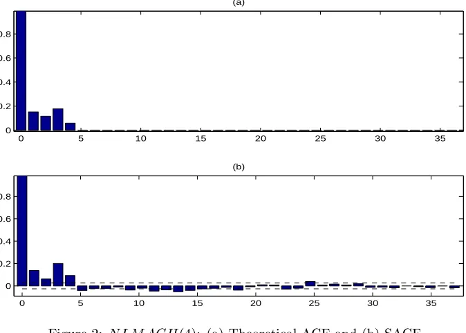
We now should be able to identify empirially the value of q by means of the sample autoorrelation funtion of the proess's squares. In order to illustratethis,wesimulatedaNLMACH(4)andplottedboth,thesampleand thetheoretialautoorrelationfuntion.
0
5
10
15
20
25
30
35
0
0.2
0.4
0.6
0.8
(a)
0
5
10
15
20
25
30
35
0
0.2
0.4
0.6
0.8
(b)
Figure2: NLMACH(4): (a)TheoretialACFand(b)SACF
Theautoorrelationfuntionmayyieldashapethatapproximatesfairlywell the oneproposed by the stylized fats in nane theory. Yet, to ahieve this weareforedto useaNLMACH(q)withqgreaterthanunity. Analternative to this is to generalize the proess by inluding lags of h
t
[image:9.595.136.473.333.574.2]One the main statistial properties have been established, the next step is estimation. TheNLMACH(1) estimation is simple despite thefat of being ahighly non-linearmodel. Inordertoshowtheperformaneoftheestimating tehnique, wepresentaMaximum Likelihood (ML) estimate. Itworksin the samewayaswithAR CH models. TheMLestimationoftheNLMACH(q)is straightforward.Wetakeadvantageofthefatthattheonditionaldistribution isN(0;h
1=2 t
),thatis,X t
= t
N(0;h 1=2 t
),where t
isthepastinformationset 3
. Under the usual regularity onditions, we are thus able to ompute the orrespondingLikelihoodandmaximizeitusingagradientalgorithm.
WeperformedaMonteCarloExperimenttoillustratetheMLestimator. Table (1)exhibitstheestimationresultsforavarietyofparameters(bothparameters adoptthefollowingvalues: 0.25,0.50and0.75). 1,000repliationswheremade foreahase. Table (1) showsthe averages ofsuh estimationsaswellas the standardeviations
4 .
Parameters Samplesize
T=200 T=500 T=700
Æ 0
Æ 1
b Æ
0
b Æ
1
b Æ
0
b Æ
1
b Æ
0
b Æ
1 0.25 0.250 0.248 0.251 0.249 0.251 0.249
(0.04) (0.07) (0.04) (0.05) (0.02) (0.04) 0.25 0.50 0.249 0.494 0.251 0.498 0.250 0.506
(0.04) (0.12) (0.03) (0.08) (0.02) (0.07) 0.75 0.251 0.742 0.253 0.748 0.250 0.749
(0.04) (0.18) (0.03) (0.11) (0.02) (0.09) 0.25 0.501 0.249 0.500 0.246 0.500 0.249
(0.08) (0.10) (0.04) (0.06) (0.04) (0.05) 0.50 0.50 0.502 0.499 0.498 0.501 0.500 0.497
(0.08) (0.15) (0.05) (0.09) (0.04) (0.08) 0.75 0.501 0.743 0.499 0.754 0.502 0.747
(0.08) (0.20) (0.05) (0.13) (0.04) (0.10) 0.25 0.756 0.243 0.754 0.247 0.749 0.251
(0.11) (0.12) (0.07) (0.07) (0.06) (0.06) 0.75 0.50 0.753 0.504 0.751 0.492 0.749 0.502
(0.11) (0.18) (0.07) (0.11) (0.06) (0.09) 0.75 0.759 0.752 0.752 0.748 0.747 0.745
(0.12) (0.22) (0.07) (0.14) (0.06) (0.12)
Table1: MonteCarloSimulationofestimatesforaNLMACH(1);N=200,500 and700
3
t=fXt 1;Xt 2
;;X0;Vt 1;Vt 2;;V0g 4
gorithm(Matlabsdefault)aonvenientestimationanbeperformed,although itseÆeneouldbeimproved. It isurioustonotiethat thestandard devia-tioninreaseswiththevalueoftheparameter.
3.1 Foreasting apability of the Models
It mustbe saidthat our proposal (NLMACH) would not be partiularly in-terestingifitwasunable to oergood foreastingapabilitiesof thevolatility of a variable. In order to study its performane in this domain, we simulate twoDGPs; an NLMACH(1) and a GARCH(1,1). Overeah simulated series we performed the estimation of both the NLMACH(1) and the GARCH(1,1) using onlyafration of the sample and onstrutedanout-of-sample foreast (oneperiodahead). Thenweaddanobservationandrebuildtheforeastuntil weuseT-1observations. Usingtheseforeastsandknowingtherealvalueswe
a
b
c
0
20%
40%
60%
80%
100%
NLMACH(1)
a
b
c
0
20%
40%
60%
80%
100%
a
b
c
0
30%
60%
90%
120%
a
b
c
0
30%
60%
90%
120%
T=200
RMSE
NLMACH
RMSE
GARCH
T=500
GARCH(1,1)
Figure3: MonteCarlo Experiment: NLMACH(1) andGAR CH(1;1) out-of-sampleforeasts: NLMACH, asesa,b and : Æ
1
=0:30, GARCH, asesa, b and: =0:30and =0:30
a)NLMACH:Æ 1
=0:15;GARCH(1,1): =0:10 b)NLMACH:Æ
1
=0:30;GARCH(1,1): =0:30 b)NLMACH:Æ
1
=0:45;GARCH(1,1): =0:50
omputetheRootMean SquareErrorforeahspeiationandthen ompute the ratio:
RMSE
NLMACH(1) RMSE
GARCH(1;1)
. We repeat the latter experiment 1000 times and showtheresults(averages)ingure(3)
5 . 5
(rst row of gure)the NLMACH(1) speiations foreasts outperforms the GARCH(1,1)s foreastsbut theinverse is notompletely true(seond rowof gure).IftheDGPisaGARCH,thereareseveralaseswheretheNLMACH(1), evenifitisthewrongspeiation,yieldsbetterforeasts.
3.2 Appliation to Exhange Rates
InordertoexaminetheNLMACHperformaneusingrealmarketdata,inthis setionweestimatetheNLMACH(1)modelandompareitwiththeAR CH(1) and GAR CH(1;1) proesses. In addition we estimate the AR CH(1) model assuming a Student-t distribution in order to apture the fat tails frequently observed in nanial returns. Eight major urrenies are employed for this exerise
6
. Daily exhange rate returnsfrom January 2,1991 to Deember29, 1995 are alulatedby taking the rst log dierene orrespondingto atotal of1,303observationsforeahurreny. Inpartiulartheexhangeratesunder examinationaretheAustralianDollar(AUS),BritishPound(GBR),Canadian Dollar (CAN), Duth Guilder (NLG), Frenh Fran (FRA), German Dmark (DEU),JapaneseYen(JPY)andSwissFran(CHF). Desriptivestatistisare showninTable(2)below.
Curreny Mean Median StdDev. Min. Max. Skew. Kurt. AustralianD. 0.0013 -0.0117 0.1997 -0.6954 0.8527 0.4171 1.6811
BritishP. 0.0075 -0.0079 0.2906 -1.2548 1.4271 0.3502 2.5506 CanadianD. 0.0055 0.0033 0.1213 -0.7040 0.5911 0.0320 2.7627 DuthG. -0.0016 -0.0083 0.3179 -1.2581 1.3060 0.0917 1.6173 FrenhF -0.0012 -0.0019 0.3004 -1.1734 1.1519 0.0700 1.6761 GermanM. -0.0013 -0.0115 0.3190 -1.2578 1.3476 0.1233 1.6865 JapaneseY. -0.0088 -0.0087 0.2828 -1.4727 1.4014 -0.2492 3.3761 SwissF. -0.0030 0.0000 0.3470 -1.6933 1.3517 -0.0223 1.5817
Table2: Statistialharateristisoftheexhangeratetime series
Tables3,4,5and6presenttheestimationresultsforeahurrenyforseveral modelspeiations. Dierentordersoftheproesswereinvestigated. The NL-MACH(1)washosenaordingtotheAkaikeInformationCriterion(AIC)and theShwartzBayesianCriterion (SBC).Theoptimization algorithmemployed in the estimations was the BFGS and all theprograms are written in RATS. Using robust standard errors it is observed that apart from the interept all estimatedparametersarehighlysigniant{seeÆ
1 andÆ
2
ineahpanel 7
. optimalpreditions[℄".Havingsaidthis,weshouldkeepinmindthemanylimitationsof timeseriesforeastingperformane.
6
ThedatahasbeenextensivelyexaminedbyFransesandvanDijk(2000)forthissubsample andfromDeember1979. Thedataisavailableintheauthors'website.
7
NotethatÆ 1
isassoiatedtoeithertheNonlinearorARCHeetrespetively,whereas Æ
2
NLMACH ARCH GARCH ARCH-t NLMACH ARCH GARCH ARCH-t EstimatedCoeÆients
C 0:0019 0:0019 0:0046 0:0056 0:0011 0:0010 0:0070 0:0036 (0:0079)
a
(0:0074) (0:0080) (0:0093) (0:0093) (0:0098) (0:0074) (0:0082) Æ
0
0:0794 0:0794 0:0032 0:0502 0:0992 0:0986 0:0039 0:0669 (0:0030) (0:0055) (0:0006) (0:0027) (0:0037) (0:0034) (0:0007) (0:0025) Æ
1
0:0212 0:2138 0:0715 0:1620 0:0204 0:1781 0:0575 0:1309 (0:0035) (0:0466) (0:0097) (0:0289) (0:0035) (0:0271) (0:0083) (0:0281) Æ
2
0:8967 0:9098
(0:0022) (0:0015)
V b
5:4836 6:1327
(0:4327) (0:7747)
DeisionCriteria L()
867:34 866:99 894:99 804:94 746:01 746:21 763:93 934:56 AIC
d
8753:71 8753:18 8796:28 8659:16 8558:86 8559:20 8591:54 8852:14 SBC
e
8769:20 8768:67 8816:94 8679:82 8574:35 8574:69 8612:20 8872:79
Table3: ModelAdjustmentfortheDuthguilderandtheSwissFran.*,**Signiantatthe1%and10%levelrespetively. a RobustStandarderrorsinparenthesis.
b
Shapeparameter.
Optimizaedlikelihoodvalue. d
AIC=AkaikeinformationCriterion and
e
SBC=ShwartzBayesCriterion
NLMACH ARCH GARCH ARCH-t NLMACH ARCH GARCH ARCH-t EstimatedCoeÆients
C 0:0043 0:0039 0:0057 0:0062 0:0016 0:0016 0:0039 0:0058 (0:0081)
a
(0:0079) (0:0070) (0:0070) (0:0083) (0:0081) (0:0078) (0:0079) Æ
0
0:0745 0:0745 0:0024 0:0449 0:0796 0:0796 0:0033 0:0507 (0:0025) (0:0051) (0:0017) (0:0038) (0:0028) (0:0029) (0:0018) (0:0017) Æ
1
0:0153 0:1749 0:0596 0:1405 0:0217 0:2180 0:0711 0:01618 (0:0032) (0:0459) (0:0189) (0:0269) (0:0035) (0:0319) (0:0200) (0:0253) Æ
2
0:9135 0:8969
(0:0348) (0:0337)
V b
5:1436 5:5298
(0:6332) (0:4059)
DeisionCriteria L()
931:73 931:12 962:74 735:18 863:72 863:23 888:54 808:74 AIC
d
8846:30 8845:45 8890:63 8541:95 8748:29 8747:56 8786:93 8665:25 SBC
e
8861:79 8860:94 8891:29 8562:61 8763:79 8763:05 8807:59 8685:91
Table4: ModelAdjustmentfortheFrenhFranandtheGermanMark. *,**Signiantatthe1%and10%levelrespetively. a RobustStandarderrorsinparenthesis.
b
Shapeparameter.
Optimizaedlikelihoodvalue. d
AIC=AkaikeinformationCriterion and
e
SBC=ShwartzBayesCriterion
NLMACH ARCH GARCH ARCH-t NLMACH ARCH GARCH ARCH-t EstimatedCoeÆients
C 0:0065 0:0062 0:0098 0:0046 0:0059 0:0059 0:0025 0:0029 (0:0073)
a
(0:0076) (0:0080) (0:0065) (0:0032) (0:0031) (0:0032) (0:0029) Æ
0
0:0702 0:0693 0:0020 0:0347 0:0123 0:0119 0:001 0:0067 (0:0022) (0:0018) (0:0014) (0:0020) (0:0004) (0:0004) (0:0001) (0:0004) Æ
1
0:0089 0:1286 0:0484 0:0751 0:0024 0:1992 0:0517 0:1178 (0:0021) (0:0212) (0:0164) (0:0219) (0:0004) (0:0252) (0:0152) (0:0281) Æ
2
0:9251 0:9404
(0:0279) (0:0185)
V b
3:8234 4:3438
(0:3451) (0:4418)
DeisionCriteria L()
1005:55 1006:56 1045:43 616:82 2100:63 2102:25 2139:88 451:57 AIC
d
8944:88 8946:19 8997:17 8319:99 8897:44 9898:43 9923:38 7912:92 SBC
e
8960:38 8961:68 9017:83 8335:65 9912:94 9913:93 9944:04 7933:58
Table 5: Model Adjustment for the Japanese Yen and the Canadian Dollar. *,** Signiant at the 1% and 10% level respetively.
a
Robust Standard errors in parenthesis. b
Shape parameter.
Optimizaed likelihood value. d
AIC =Akaike in-formationCriterionand
e
SBC=ShwartzBayesCriterion
NLMACH ARCH GARCH ARCH-t NLMACH ARCH GARCH ARCH-t EstimatedCoeÆients
C 0:0026 0:0020 0:0015 0:0041 0:0003 0:0001 0:0011 0:0061 (0:0078)
a
(0:0076) (0:0069) (0:0066) (0:0050) (0:0056) (0:0055) (0:0050) Æ
0
0:0701 0:0672 0:0008 0:0329 0:0367 0:0367 0:0025 0:0206 (0:0022) (0:0019) (0:0005) (0:0020) (0:0012) (0:0011) (0:0023) (0:0011) Æ
1
0:0144 0:2138 0:0507 0:1490 0:0032 0:0813 0:0595 0:0723 (0:0025) (0:0294) (0:0143) (0:0321) (0:0014) (0:0228) (0:0355) (0:0239) Æ
2
0:9403 0:8794
(0:0187) (0:0903)
V b
3:8423 4:4480
(0:3606) (0:4853)
DeisionCriteria L()
975:20 979:79 1052:46 655:30 1441:20 1441:02 1457:70 219:87 AIC
d
8905:26 8911:33 9005:84 8393:00 9410:28 9410:13 9427:01 6981:21 SBC
e
8920:76 8926:83 9026:50 8413:89 9425:78 9425:62 9447:67 7001:87
Table 6: Model Adjustment for the British Pound and the Australian Dollar. *,** Signiant at the 1% and 10% level respetively.
a
RobustStandard errorsin parenthesis. b
Shapeparameter.
Optimizaedlikelihood value. d
AIC =Akaike infor-mationCriterionand
e
SBC=ShwartzBayesCriterion
andSBCriteriaprovidemixed evidene. Forinstaneaordingto these ri-teria NLMACH(1) is preferred to the AR CH(1) for the Swiss Fran, the Japanese Yen, the Canadian Dollar and the British Pound. When the NL-MACH(1)is omparedtoGARCH(1,1)it isobservedthat inallasesthe NL-MACH(1)ispreferredtoGARCH(1,1). Surprisingly,aordingtotheseriteria, theARCH(1)modelisalsopreferredtoGARCH(1,1). However,weneedtobe autious about using these riteria to disriminate between models. The use ofthesestatistismightnotbeentirelyappropriatesinethetwotypesof pro-esseshaveadistint nonlinearnature. Moreover,thestatistial propertiesof AICandSBChavenotbeeninvestigatedforthelassofnonlinearmodelshere proposed. UsingtheOptimized Likelihoodvalueastheseletionriterion, the GARCH(1,1) is themodel that ts the data best. This howeveris not nees-sarilybad newsfortheNLMACH(1) sineitonlyindiates that GARCH(1,1) aptures well a spei type of onditional heteroskedastiity. One last ase hasbeeninvestigated: theAR CH(1)with at-distributionin order toapture thefattailsandnon-normalityof thedata
8
. It turnsoutthat,asindiatedby theAIC and SBC, this model isstrongly preferredto allother speiations inluding the NLMACH(1) with the only exeption of the Swiss Fran. As wehavealreadyshown,ourNLMACH(1)modelreproduesthefattailsquite naturallywithout the need of imposing a dierent onditional distribution to repliatethisbehavior. However,assuggestedbytheseresults,imposinga on-ditionaldistributiondierentthananormalmight aptureotherpropertiesof thedata. Forinstane, itmightbethat thesoureof non-normalityisdue to theexisteneofoutliers;thisfeatureisnotobviouslytakenintoaountbythe NLMACH(1)model.
8
Thispaperhaspresentedanewmodel,deeplyinspiredbytheNon-Linear Mov-ing Average models, but with the approah typiallyused when dealingwith onditionallyheteroskedastimodels. Averysimplespeiationmodiation solvesthetypialproblemsofthislass. NLMACH hassimplestatistial prop-ertiesandiseasytoestimate. Itshouldindeedbeseenasanewinstrumentto dealwithheteroskedastiity. Severaltoolspresentedhereaimtofulllthis pur-pose. Ononehand,NLMACHanbeeasilyestimatedbyML. Thisestimation tehniqueprovedtobeeÆientandreliable. Ontheotherhand,thetheoretial results,suhastheautoorrelationfuntionformofthesquaredproessshould failitate identiation, and provide statistial evidene of either thepresene orthe abseneofNLMACH behavior. forsomepartiularases(speiedin theDGPsandthesamplesizeoftheMonteCarloexperiments)NLMACH(1)' foreasting apabilities outperform
9
the ones yielded by GAR CH(1;1) even whenthetrueDGP isaGAR CH(1;1).
Thisnewspeiationwillhavetoompetewiththemanyvariants belong-ingto theAR CH lass. Suh ompetitorsvary in omplexityand robustness. NLMACHistherepliationoffattails;theestimationresultsindiatehowever thatthisproessispreferredtoARCHmodelsusingastudent-tasonditional distributiononlyin onease{theSwissFran. TheNLMACH model,despite its simpliity, still oers extremely interesting harateristis. All in all, the relativeevideneinfavorofNLMACHvariesinomplexityandrobustnessand all we hope is to inrease empirial interest for Non-Linear Moving Average models,whihhavebeenvirtuallynegletedalongthepastdeades.
9
Bollerslev, T. (1986): \Generalized Autoregressive Conditional Het-eroskedastiity,"Journalof Eonometris,31,309{28.
Bollerslev, T., R. Chou, and K. Kroner (1992): \ARCH modeling in Finane: a Review of Theory and EmpirialEvidene," Journal of Eono-metris,52, 5{59.
Boulier,J.(1994):Modelisation ARCH:TheoriesStatistiquesetAppliations dans leDomaine dela Finane.Ellipses.
Engle,R.(1982a): \AutoregressiveConditionalHeteroskedastiitywith Esti-mates oftheVarianeoftheU.K.Ination,"Eonometria,50,987{1008. Engle, R., D. Lilien, and R. Robins (1987): \Estimating Time Varying
Risk Premia in the Term Struture: the ARCH-M Model," Eonometria, 55,391{407.
Franses, P., and D. van Dijk (2000): Non-Linear Time Series Models in Empirial Finane.Cambridge.
Granger, C. W. (1998): \Overviewof Nonlinear TimeSeries Speiations in Eonomis,"UCSD,rstdraft.
Granger, C.W., and A. Andersen (1978): AppliedTime SeriesAnalysis. AademiPress,pp.25-38EditedbyDavidF.Findley.
Granger,C.W.,andT.Terasvirta(1993):ModellingNonlinearEonomi Relationships.OxfordUniversityPress.
Gu
egan, D. (1994): Series Chronologiques Non Lineaires a Temps Disret. Eonomia.
Nelson,D.(1991): \ConditionalHeteroskedastiityinAssetReturns: ANew Approah,"Eonometria,59,347{70.
Robinson, A. (1977): \The Estimation of a Non Linear Moving Average Model,"Stohasti Proessesandtheir Appliations,1,81{90.