ISSN: 1992-8645 www.jatit.org E-ISSN: 1817-3195
144
COMPARISON OF SOFTWARE RELIABILITY ANALYSIS
FOR BURR DISTRIBUTION
1
Dr. G. SRIDEVI, 2Dr. C.M. SHEELA RANI 1
Professor, Dept. of CSE, K.L.University, Vaddeswaram, India. 2
Assoc. Professor, Dept. of CSE, K.L.University, Vaddeswaram, India.
E-mail: [email protected], 2 [email protected]
ABSTRACT
This model is for Burr type distribution with three parameters which is discussed in two versions - the Burr type III and Burr Type XII. In this paper, we compare the performance of two versions of the suggested model is tested on five real time software failure data sets. The versions perform with variable accuracy, which suggest that no universal “best” among the two versions of the model could be attained.
Keywords: Burr type III Model; Burr type XII Model; NHPP; ML Estimation;
1. INTRODUCTION
The important quality characteristic of software is software reliability, which can evaluate and estimate the operational quality of a software system during its development. Software Reliability is the probability of failure free operation of software in a specified environment for a specified period of time (Lyu, 1996) (Musa et al., 1987). SRGM is a mathematical model of how the software reliability improves as faults are detected and required (Quadri and Ahmad, 2010). Among all SRGMs developed so far a large family of stochastic reliability models based on a Non-Homogeneous Poisson Process known as NHPP reliability model has been widely used. The main objective is to develop a reliability growth model that can be used to provide quantitative measure for software performance assessment. There is several software reliability growth models exist, one can predict the reliability of software and the number of errors in the software systems. During the past three decades research on software reliability engineering has been conducted and developed numerous statistical models for estimating software reliability. Most existing models for predicting software reliability are based purely on the observation of software product failures where they require a considerable amount of failure data to obtain an accurate reliability prediction. The concept of Probability, distribution function,
probability distribution plays an important role in building the software reliability growth model.
2. RELATED RESEARCH
Burr type XII distribution was first introduced in 1942 by Irving W. Burr. Since the corresponding density functions have a wide variety of shapes, this system is useful for approximating histograms. The Burr XII (BXII) distribution, having logistic and Weibull as special sub models, is a very popular distribution for modelling lifetime data and for modelling phenomenon with monotone failure rates. It has been applied in the field of reliability studies and failure time modelling. This section presents the theory that underlies the proposed distributions and maximum likelihood estimation for complete data. If ‘t’ is a continuous random
variable with pdf:
f t
( ; ,
θ θ
1 2,...,
θ
k)
. Where1
,
2,...,
kθ θ
θ
are k unknown constant parameters which need to be estimated, and CDF:F t
( )
Where, the mathematical relationship between the
PDF and CDF is given by:
f t
( )
d F t
( ( ))
dt
=
. LetISSN: 1992-8645 www.jatit.org E-ISSN: 1817-3195
145 cumulative distributive function. The failure intensity function
λ
( )
t
in case of the finite failureNHPP models is given by:
λ
( )
t
=
aF t
'( )
(Pham, 2006).3.NHPP MODEL
There are several software reliability growth models available for use according to probabilistic assumptions. The first one is the Markovian model which is the failure process represented by Markov. The second one is the fault counting model which describes the failure phenomenon by stochastic process like Homogeneous Poisson Process (HPP), Non Homogeneous Poisson Process (NHPP) and Compound Poisson Process. The Non Homogenous Poisson Process (NHPP) based software reliability growth models are proved to be quite successful in practical software reliability engineering [4]. Model parameters can be estimated by using maximum Likelihood Estimation (MLE). The formulation of NHPP model is described in the following lines.
A software system is subject to failures at random times caused by errors present in the system. Let
{
N t t
( ),
≥
0
}
be the cumulative number of software failures by time ‘t’, where t is the failure intensity function, which is proportional to the residual fault content. As there will be no errors at t=0 we have( ) 0 N t =
Let
m t
( )
represent the expected number of software failures by time‘t’. As the expected number of errors remaining in the system is finite, the mean value functionm t
( )
is finite.0,
0
( )
,
t
m t
a t
=
=
→ ∞
Where ‘a’ is the expected number of software errors to be eventually detected.
Suppose
N t
( )
is known to have a Poisson probability mass function with parametersm t
( )
i.e.,
Where N(t) is the cumulative number of failures observed by time ‘t‘, N(t) can be modeled as a Poisson Process with a time dependent failure rate. Thus the stochastic behavior of software failure phenomena can be described through the N(t) process. Various time domain models have developed in the literature (Kantam & Subbarao, 2009) that describes the stochastic failure process by an NHPP which differ in the mean value function
m t
( )
.4. DESCRIPTIONS OF BURR TYPE MODELS
In this section, we propose two variations of Burr type distribution models. The Burr distribution has a flexible shape and controllable scale and location which makes it appealing to fit to data. It is frequently used to model insurance claim sizes [5].
4.1 Burr type III Model Development
The mean value function of Burr type III model is given by [17]
(t)
a 1
c bm
=
+
t
−
−(1)
To assess the software reliability, the parameter values ‘a’, ‘b’ and ‘c’ are estimated from software failure data. To estimate the parameter values for the Burr type III model, expressions are derived as mentioned below. Assuming that the data are given for the occurrence times of the failures or the times of successive failures, i.e., the realization of random variables Tj for j = 1, 2,..,n.
Parameter Estimation – Mathematical Derivation for Burr type III model
Given the recorded data on the time of failures, the Log likelihood function (LLF) takes on the following form[17]:
[
]
1
log
( )
( )
n
i n i
LLF
λ
t
m t
=
=
∑
−
(2)
{
( )
}
[
( ) .e
]
( ),
0,1, 2,...
!
n m t
m t
P N t
n
n
n
−
ISSN: 1992-8645 www.jatit.org E-ISSN: 1817-3195
146
(
)
11 1
log
1
1
nb c b c c i n i i
abc
a
LogL
t
t
+t
− + −=
=
−
+
+
∑
(3)(
)
11
log
log
log
(
1) log
(
1) log(1
)
b c n n c i i i
a
LogL
t
a
b
c
c
t
b
t
− − =
−
=
+
+
+
+
− +
−
+
+
∑
(4)Accordingly parameters ‘a’, ‘b’ and ‘c’ would be solutions of the equations
0
LogL
a
∂
=
∂
⇒ =
a
n
(
1
+
t
n−c)
b(5)
0
LogL
b
∂
=
∂
(
1)
(
1)
1
log 1
log 1
n
i n
i
n
b
t
−n
t
−=
⇒ =
+
−
+
∑
(6)
The value of the parameter ‘c’ is estimated by Newton-Raphson iterative method using
1 '
( )
( )
i i i ig c
c
c
g c
+
= −
whereg c
( )
and'
( )
g c
areexpressed as
0
LogL
c
∂
=
∂
1log(t )
( )
1
2
log
1
1
n c n n i c i in
n
g c
t
c
t
t
=−
⇒
=
+ +
+
− +
+
∑
(7) 2 2
0
LogL
c
∂
=
∂
(
)
2 ' 2 2 2 2 1(log t )
( )
(1
)
2
log
(
1)
c n n c n c n i i c i in
t
n
g c
t
c
t
t
t
=⇒
=
−
−
+
+
∑
(8)
The value of ‘c’ in the above equations (7) & (8) can be obtained using Newton-Raphson iterative method.
4.2 Burr Type XII Model Development
The Cumulative distributive function (CDF) for Burr type XII is given by[18]
(
)
1 0
( )
( )
1
1
c bm t
=
λ
t dt
=
a
− +
t
−
∫
=
a F t
( )
The Probability Density Function (PDF) of Burr XII distribution are given, respectively by
(
)
1 1( )
( )
1
c b ccbt
t
a
a f t
t
λ
− +
=
=
+
The mean value function of Burr type XII model is given by
(
)
( )
1
1
c b,
0
m t
=
a
− +
t
−
t
≥
(9)Parameter Estimation – Mathematical Derivation for Burr type XII model
We conduct an experiment and obtain N
independent observations
t t
1, ,...,
2t
n. The likelihood function for time domain data (Pham, 2003) is given by[18]( ) 1
( )
n m t i iL
e
−λ
t
=
ISSN: 1992-8645 www.jatit.org E-ISSN: 1817-3195
147
1
1 (1 ) 1
1
(1
)
.
c b b N a t c c i i i
L
abct
t
e
− + − − + − =
=
∏
+
1(1
)
(
1) log
(
1) log(1
)
c b
n
c
i i i
LogL
a
a
t
Log a
Log b
Log c
c
t
b
t
− =
= − +
+
+
+
+
+
−
−
+
+
∑
Taking the Partial derivative with respect to ‘a’ and equating to ‘0’.
(i.e.,
Log L
0
a
∂
=
∂
).
(1
)
(1
)
1
c b c b
n
t
a
t
+
∴ =
+
−
(11)The parameter ‘b’ is estimated by iterative Newton
Raphson Method using , Where
′ are expressed as follows.
0
1
1
log
1
( )
log(t
1)
(
1)
1
n i b
i
n
Log L
t
n
g b
b
t
b
=
∂
=
=
+
+ −
+
∂
+
−
∑
(12)
2 ' 2
( )
LogL
0
g b
b
∂
=
=
∂
(
)
2 ' 2 2 21
(
1) log(
1)
1
( )
log
1
1
1
b b
LogL
t
t
g b
n
b
t
t
b
∂
=
= −
+
+
+
∂
+
+
−
(13)
The parameter value of ‘c’ is estimated by iterative Newton Raphson Method using
Where ′ are expressed as
0
1 1
( )
log( )
(1
)
2log( )
log
(1
)
c c n n i i ci i i
LogL
n
g c
t
c
t
t
n
t
t
c
=t
=∂
=
=
−
+
∂
+
−
+
+
∑
∑
(14)
′
0
2 '2 2 2
2 1
log
( )
log
(1
)
1
2 log .
log
(1
)
c c
n c
i i c
i i
Log L
nt
t
n
g c
t
c
t
c
t
t
t
t
=∂
=
=
−
∂
+
−
+
∑
(15)
Let be the time between 1 and failure of the software product. Let ! be the time up to the failure. Let us find out the probability that time between 1 and failures, i.e., exceeds a real number ‘s’ given that the total time up to the 1 failure is equal to ".
i.e.,
# $ %
&'()*
"+
, /!
.//"
0
.12 3 & .2 & 4This Expression is called Software Reliability.
5. DATA ANALYSIS
In this section we evaluate the method of performance based on the considered mean value function for five different data sets of the above form, borrowed from (Xie, 2002), (Pham, 2006), IBM (Ohba, 1984) and (SONATA , 2010).
ISSN: 1992-8645 www.jatit.org E-ISSN: 1817-3195
148 numerical methods. The parameter estimates are presented in Table I.
Table 1: Parameters Estimated through MLE
Version Datasets
No of Sam ples
Estimated Parameters
a b c
Burr Type III
NTDS 26 34.46570 1.76364 1.81
022
AT & T 22 26.83982 1.65869 1.00
000
Xie 30 33.31042 2.27009 1.37
197
SONATA 30 79.83135 6.74281 0.60
244
IBM 15 20.62478 1.71163 1.44
781
Burr Type XII
NTDS 26 26.10527 0.99889 0.99
890
AT & T 22 22.03246 0.99985 0.99
961
Xie 30 30.04080 0.99982 0.99
961
SONATA 30 30.01639 0.99995 0.99
992
IBM 15 15.05104 0.99953 0.99919
6. METHOD OF PERFORMANCE ANALYSIS
The performance of SRGM is judged by its ability to fit the software failure data. The term goodness of fit denotes the question of “How good does a mathematical model fit to the data?”. In order to validate the model under study and to assess its performance, experiments on a set of actual software failure data have been performed. The performance evaluation of software reliability growth model is generally measured with sum of square errors (SSE) and correlation index of regression curve equation (R-squared). Among them, the model performance is better when SSE is smaller and R-square is close to 1.
SSE is used to describe the distance between actual and estimated number of faults detected totally, which is defined as
(
)
21
( )
n
i i i
SSE
y
m t
=
=
∑
−
Where n denotes the number of failure samples in failure data set,
i
y
denotes the number of faultsobserved to the moment
i
t
, andm t
( )
i denotes theestimated number of faults detected to the time
i
t
according to the proposed model. The model can provide a better goodness-of-fit when the value of SSE is smaller.
The equation of calculating the value R-square is written as:
2 1
2 1
( )
n
i i
n
i i
y m t
R
squared
y y
− =
− =
−
−
=
−
∑
∑
Where
y
−
denotes the mean value of faults
detected. The model can provide a better goodness-of-fit when the value of R-squared is close to 1.
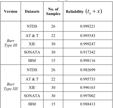
[image:5.612.307.532.430.646.2]We compare the reliabilities of both Burr type III and Burr type XII software failure data sets that are presented in Table II and method of performance analysis is given in Table III.
Table 2: Reliabilities Of Different Datasets
Version Datasets No. of
Samples Reliability
(
t
n+
x
)
Burr Type III
NTDS 26 0.999221
AT & T 22 0.995543
XIE 30 0.999247
SONATA 30 0.917342
IBM 15 0.998116
Burr Type XII
NTDS 26 0.982699
AT & T 22 0.995733
XIE 30 0.996163
SONATA 30 0.997002
ISSN: 1992-8645 www.jatit.org E-ISSN: 1817-3195
149 Table 3: Method Of Performance Analysis
Version Datasets SSE R-Squared
Burr Type III
NTDS 207873.68 0.893299
AT & T 1795108.55 1.114142
XIE 2643026 0.937608
SONATA 29162065.81 2.213800
IBM 272918.63 1.380632
Burr Type XII
NTDS 237127.57 1.165665
AT & T 1838993.61 1.161281
XIE 2684707.24 0.968715
SONATA 31286816.43 2.426521
IBM 290810.07 1.537804
From Table III it can be seen that the value of SSE is smaller and the value of R-squared is more close to 1. The results indicate that our NHPP Burr type III & Burr type XII model based on fault detection rate fits the data in the given datasets, best and predicts the number of residual faults in software most accurately.
7. CONCLUSION
Software reliability growth model can estimate the optimal software release time and the cost of testing efforts [13]. And SRGM can help project managers to determine the testing resources and manpower needed to achieve desired reliability requirements. So more accurate model is needed to decrease the testing cost and increase the profit of releasing software [11][14][15]. In this paper the fault detection rate is calculated with the number of faults remaining in the software. Considering the two factors jointly the fault detection rate is more realistic and accurate. Moreover, we have discussed the performances of 5 datasets using Burr type III & Burr type XII SRGMs. The experiment result shows that the NTDS data set of Burr type III can provide a better goodness-of-fit compared with other datasets are given in Table III. The reliability of the model over Xie data of Burr type III is high among the data sets which were considered.
REFERENCES:
[1] Kimura, M., Yamada, S., Osaki, S., 1995. ”Statistical Software reliability prediction and its applicability based on mean time between failures”. Mathematical and Computer Modelling Volume 22, Issues 10-12, Pages 149-155.
[2] Pham, H. (2005), “A Generalized Logistic Software Reliability Growth Model”, Opsearch, Vol.42, No.4, 332-331.
[3] Lyu, M.R., (1996), “Handbook of Software Reliability Engineering”, MCGraw-Hill, New York.
[4] Musa, J.D., Iannino, A., Okumoto, k., 1987. “Software Reliability: Measurement Prediction Application”. McGraw -Hill, New York.
[5] Hee-cheul Kim., “Assessing Software Reliability based on NHPP using SPC”, International Journal of Software Engineering and its Applications, vol.7,No.6 (2013), pp.61-70.
[6] Pham. H., 2003. “Handbook Of Reliability Engineering”, Springer.
[7] Pham. H., 2006. “System software reliability”, Springer.
[8] Goel, A.L., Okumoto, K., 1979. Time-dependent error detection rate model for software reliability and other performance measures. IEEE Trans. Reliab. R-28, 206-211.
[9] Quadri, S.M.K and Ahmad, N., (2010), “Software Reliability Growth Modelling with new modified Weibull testing-effort and optimal release policy”, International Journal of Computer Applications, Vol.6, No.12.
[10] Xie, M., Yang, B. and Gaudoin, O. (2001), “Regression goodness-of-fit Test for Software reliability model validation “, ISSRE and Chillarege Corp.
[11] C. Y. Huang and C.T. Lin, “Analysis of software reliability modeling considering testing compression factor and failure-to-fault relationship, “IEEE Trans. On Computers, vol. 59, no. 2, pp. 283-288, Feb. 2010.
[12] Tao Li and Kaigui Wu, “A NHPP Software Reliability Growth Model Considering Learning Process and Number of Residual Faults”
[13] Huang CY, Kuo SY, Lyu MR, “An Assessment of Testing-Effort Dependent Software reliability Growth Models,” IEEE Computer, 2007, 56(2): 198-211.
ISSN: 1992-8645 www.jatit.org E-ISSN: 1817-3195
150 Network Environment”, IJACT: International journal of Advancements in Computing Technology, Vol. 4, No. 1, pp.136-144, 2012.
[15] Xu Jian, Yan Han, Li Qianmu, “A Methodology for Software Reliability Risk Assessment”, JCIT: Journal of Convergence Information Technology, Vol.6, No. 4, pp. 188-200, 2011.
[16] Tao Li and Kaigui Wu, “A NHPP Software Reliability Growth Model Considering Learning Process and Number of Residual Faults”
[17] Ch. Smitha Chowdary, Dr. R.Satya Prasad, K.Sobhana, “Burr type III Software Reliability Growth Model”, IOSR Journal of Computer Engineering, Volume 17, Issue 1, pp 49-54.
[18] R.Satya prasad, K.V.Murali Mohan, G.Sridevi, “Burr type XII Software Reliability Growth Model”, International Journal of Computer Applications”, Volume 108-No, 16 December 2014.
[19] Asoka. M., (2010), “Sonata Software limited”, Data set, Bangalore.