ENHANCED PLANTED(ℓ,D) MOTIF SEARCH PRUNE ALGORITHM FOR PARALLEL ENVIRONMENT

ISSN: 1992-8645 www.jatit.org E-ISSN: 1817-3195

DIFFERENTIAL EVOLUTION (DE) ALGORITHM TO

OPTIMIZE BERKELEY - MAC PROTOCOL FOR WIRELESS

SENSOR NETWORK (WSN)

1_{ALAA KAMAL,} 2_{M.N. MOHD. WARIP,} 3 _{MOHAMED ELSHAIKH}

, 4 R.BADLISHAH

1,2,3,4

Embedded Network and Advanced Computing Research Cluster, School of Computer and Communication engineering, University Malaysia Perlis, Level 1, Pauh Putra Main Campus, 02600, Arau,

Malaysia

E-mail: [email protected], [email protected] ,

3

[email protected] , [email protected]

ABSTRACT

The Energy efficient being the main constraint for wireless sensor networks (WSN) became an important area of interest for various researches in WSN. A lot of work on conservation power consumption at a different layer of protocols is present till date, of which energy conservation at a Medium access control (MAC) layer is catching a lot of attention. Generally, The energy consumption it is a main critical factor affecting the operational lifetime of individual nodes and the entire network. The energy consumption in medium access control (MAC) for wireless sensor network (WSN) affected by many reasons collision, overhearing, Idle Listening, Control Overhead. The optimizing power consumption is a challenge to prolong lifetime network. In this paper, we minimize the power consumption of the B-MAC protocol for wireless sensor network (WSN) by using Differential Evolution (DE) algorithm. Simulation experiments are carried out on the discrete event simulator OMNET++ for the purposes of this research paper. Moreover, the experimental analysis shows the improvement the energy consumption of (DE-BMAC) can be conserved about (58.6%) more than B-MAC without affect the network performance.

Keywords: Berkeley MAC Protocol, Differential Evaluation (DE), Optimization, Power Consumption,

WSN

1. INTRODUCTION

MAC protocols draw a lot of attention due to their effect on the lifetime of wireless Sensor Network (WSN). Sensor nodes are driven by batteries which have a limited lifetime. Also, these nodes are deployed in the harsh environment where their change or recharge becomes difficult. An energy efficient design and implementation of MAC protocol can reduce the battery consumption and increase the sensor nodes lifetime. Traditional MAC protocols are cannot solve the energy efficient for WSN .So, we need modification in MAC protocols to minimize the power consumption and maximum Network performance[1]. In Berkeley-MAC protocols there many parameters can affect the power consumption and overall performance. Some parameters are listed for B-MAC protocol, slot duration, Check interval, Bit rate, max transmission power. In literature, there has an amount of researches MAC

ISSN: 1992-8645 www.jatit.org E-ISSN: 1817-3195

energy-efficient configurations. The experimental analysis shows that significant improvements over the standard configuration can be attained in terms of energy savings (up to 30%) without degrading the QoS. In 2011, J. Toutouh et al. [5] Assess between OLSR and DE-OLSR by using IEEE 802.11p definition and considering different urban areas sizes, traffic densities, and workloads. The QoS has been measured using four metrics: PDR, NRL, E2ED, and RPL. This comprehensive performance evaluation shows that DE-OLSR is better-suited for VANETs than the standard version, improving its resource consumption and scalability. J. Toutouh et al. [6] Deals with the optimal parameter setting of the OLSR, a well-known mobile ad hoc network routing protocol, by defining an optimization problem. Using Differential Evolution (DE), Particle Swarm Optimization (PSO), Genetic Algorithm (GA), Simulated Annealing (SA) algorithms in order to find automatically optimal configurations of this routing protocol. In the literature for designing and implementation of routing protocols that aimed to reduce the energy consumption, however, a few works are dedicated to optimizing and analyzing the affect the parameters MAC protocols set on the energy consumption for wireless sensor network (WSN). In This paper we define an optimization power consumption to the Berkeley-MAC (B-MAC) protocol, obtaining the configuration that with a specific characteristic of wireless sensor network (WSN). Furthermore, the evaluated done by using Differential Evaluation (DE) algorithm. Chosen Differential Evaluation (DE) algorithm because is a simple and presented wide solvers for Real-valued parameter. Simulation experiments are done to optimize and analyze B-MAC protocol parameters set against energy consumption, throughput, and packet delivery ratio (PDR). Moreover, concern to minimize the power consumption, and maximize the Throughput and packet delivery ratio (PDR). The paper is organized as follow: section 2 gives an overview of Differential Evaluation (DE). Section 3 describes the proposed framework of this work. Section 4 describe the Experimental setting. The Result and Discussion in section 5 and we conclude this paper in Section 6.

2

Differential Evolution (DE) has recently emerged as a simple and efficient algorithm for global optimization over continuous spaces. DE it is much easier to implement and applies a kind of

differential mutation operator on parent chromosomes to generate the offspring. Since its inception in 1995, DE has pulled the attention of many researchers all over the world, resulting in a lot of variant of the basic algorithm, with improved performance[7]:

2.1 Differential Evolution Algorithm (DE)

DE is a simple and easy evolutionary algorithm. DE it works through steps a simple cycle of stages, Below we explain each step separately[8][9]

2.1.1 INITLIZATION

DE searches for an optimum point in a D-dimensional continuous space. It begins with a randomly initiated population of NP D – dimensional Real-valued parameter vectors. Each vector, also known as the genome, forms a candidate solution to the multidimensional optimization problem. Appear subsequent generations in DE by discrete time steps like t = 0, 1,2 ...t, t+1 the successive generations are represented by G, G+1, G+2….... g, g+1 . The parameter vectors are likely to be changed over different generations, we adopt the following notation for representing the i- th vector of the population at the current generation (at time t = t) as:

Xi (t) = [xi, 1 (t), xi, 2 (t)... xi, D (t)] Where

i = 1, 2… NP.

At the very starting of a DE run at t = 0, problem parameters or independent variables are initialized somewhere in their convenient numerical range. So, if the j-th parameter of the given problem has its lower and upper bound as Xmin, Xmax, and rand i, j

(0, 1) indicated the j-th instantiation of a uniformly distributed random number between 0 and 1 for i-th vector, then we may initialize the j-th component of i-th population members as:

ISSN: 1992-8645 www.jatit.org E-ISSN: 1817-3195

2.1.2 MUTATION

Mutation mean (biology) change a genome that has characteristics resulting from chromosomal alteration. In the evolutionary computing paradigm, mutation is also seen as a change with a random element. DE, applies not to generate increments, but to randomly sample vector differences like Δ X r2, r3 = (Xr2 – Xr3)

In DE, mutation amounts to creating a donor vector V i (t) for changing each population member X i (t),

in each generation (or in one iteration of the algorithm). To create Vi (t) for each i-th member of

the current population (also called the target vector), three other distinct parameter

Vectors say the vectors Xr1i, Xr2i, and Xr3i are

chosen randomly from the current population. Where r1i, r2i, and r3i are mutually exclusive integers

randomly chosen from the range [1, NP], which are also different from the base vector index i. These indices are randomly generated once for each mutant vector. Now the difference of any two of these three vectors are scaled by a scalar number F and the scaled difference is added to the third one whence we obtain the donor Vector V i (t), can express the process as,

V i (t), = Xr1i (t) + F (Xr2i (t)-Xr3i (t)) (1)

The mutation scheme has different kinds of DE schemes but in this research used the formula in Equation (1).

2.1.3 CROSSOVER

To increase the potential diversity of the population, a crossover operation comes into play after generating the donor vector through mutation. The DE family of algorithms can use two kinds of crossover schemes - exponential and binomial. The donor vector exchanges its body parts.

Components with the target vector Xi (t) under this operation to form the trial vector

Ui (t) = [ui, 1(t), ui, 2 (t)... ui, D (t)]

Binomial crossover is performed on each of the D variables whenever a randomly choose number between 0 and 1 is less than or equal to the CR value. The scheme may be outlined as:

Ui, j,G = Vi,j,G , If (rand i, j (0,1) ≤ CR

X,j,G , otherwise

2.1.4 SELECTION

The last phase of a DE-iteration is the “selection”. Deciding who between the target vector Xi (t) and the newly formed trial vector Ui (t) will survive to the next generation. The decision whether original Xi (t) will be retained in the population or will be replaced by Ui (t) in the next time step t+1 is entirely dependent upon the ‘survival of the fittest’ concept. If the trial vector yields a better fitness value it will replace the target vector in the next time step. Here by better fitness value we mean a lower value of the objective function in case of a minimization problem, and a higher value of the same if it is a maximization problem. The selection operation may be outlined as:

Xi (t+1) = Ui (t) if F (Ui (t)) ≤ F (Xi (t))

Xi (t) F (Ui (t)) > F (Xi (t))

Where F(X) is the function to be minimized. Any one between the target vector and its offspring survives the population size remains fixed throughout generations. The fitness of the population members either improves over generations or remains unchanged, but never deteriorates.

The selection mechanism of the classical DE algorithm. The objective function we are trying to minimize is the three dimensional sphere function given by,

F(x) =

_∑

= n

i 1

ISSN: 1992-8645 www.jatit.org E-ISSN: 1817-3195

3 PROPOSED FRAMEWORK

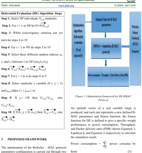
The optimization of the Berkeley – MAC protocol parameters configuration is carried out through two phases, optimization phase, and simulation phase. Figure 1 explains the main components of proposed framework for DE- Berkeley MAC protocol for WSN. Generally, the framework is consist of optimizing algorithm and evaluation procedure. Differential Evolution (DE) algorithm is used as an intelligent technique to find optimal values.

Figure 1: Optimization framework for DE-BMAC Protocol

An optimal vector of a real variable range is produced, and each one represents a new defined B-MAC parameters and fitness function. the fitness function for DE is defined to give a specific weight performance to power consumption, Throughput, and Packet delivery ratio (PDR) shown Equation 3, Equation 4, and Equation 5 respectively to calculate the simulation result.

Power consumption =

_∑

= n

i 1

power consume by

hosts (3) Throughput (bit) = ∑ Number of packet receive* 8 /

time simulation (4)

PDR= ∑ Number of packet receive / ∑ Number of packet send. (5)

4 EXPERIMENTAL SETTING

The parameters and values used to calculate the DE-BMAC explain in Table 1. Additionally, Table 2 define the DE algorithm parameters for the optimization process.

Deferential Evaluation (DE) Algorithm Steps

Step 1: Select NP individuals Xi,j,g randomly.

Step 2: For i = 1 to NP let Fi=F(Xi,j,g)

Step 3: While (convergence criterion not yet

met) do steps 4 to 10

Step 4: For i = 1 to NP do steps 5 to 10

Step 5: Select three different random indexes r0,

r1 and r2 between 1 to NP (i≠r0≠r1≠r2)

Step 6: Vi,j,g=Xr0,j,g+ F (Xr1,j,g-Xr2,j,g)

Step 7: For j = 1 to n do steps 8 to 9

Step 8: Select randomly rj variable (0 ≤ rj < 1)

and jrand index (1 ≤ jrand ≤ n)

Step 9: If rj< CR then Uj,I,g=Vj,I,g else

Uj,I,g=Xj,I,g

Step 10: If F(Ui,j) ≤ Fi (xi,j) then Xi,g+1=Ui,g else

ISSN: 1992-8645 www.jatit.org E-ISSN: 1817-3195

Table1: DE-BMAC Configuration

Main parameters

Range of values

Slot duration (s) [0.0025,0.00125, 0.0006] Bit rate (bps) [4915200, 9830400,

19660800] Check interval

(s)

[0.001 0.002, 0.004]

Max power transmission

(mw)

[1, 2, 4]

Table2: Parameters Of DE Optimization Algorithm

Parameters value

Crossover probability

(CR)

0.9

Mutation Factor (F)

0.9

According to, the steps of DE algorithm defined previously the optimum values explain in Table 3

Table 3: Optimum Values For DE-BMAC Protocol

The simulation was carried out by using OMNET++ simulator over defined wireless sensor network (WSN) scenario has been carried out based on B-MAC parameters, range values for DE-BAMC, and WSN parameters explain in Table 4

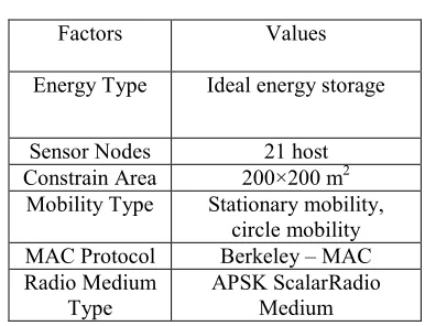
Table 4: Main Parameters Defined For OMNET++ Simulation

Factors Values

Energy Type Ideal energy storage

Sensor Nodes 21 host Constrain Area 200×200 m2

Mobility Type Stationary mobility, circle mobility MAC Protocol Berkeley – MAC Radio Medium

Type

APSK ScalarRadio Medium

5 RESULT AND DISCUSSION

The optimum value for DE-BMAC protocol carried out by using OMNET++ simulator and evaluated the result with B-MAC protocol.

Figure 2 illustrate power consumption versus the different message length used the B-MAC and DE-BMAC. It is seen the DE-BMAC outperformed the B-MAC protocol in term minimizes power consumption. However, Power consumption increased when the increased the size of message length.

Figure 2: DE-BMAC Power Consumption

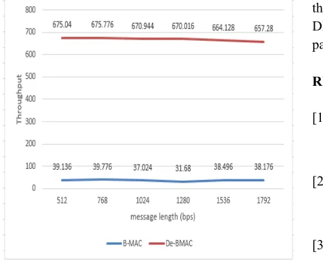
Figure 3 explain the Throughput of B-MAC protocol and DE-BMAC. In general, the performance evaluation shows that the Throughput Parameters Optimum Value

Slot Duration 0.00107 s

Bit Rate 34406400bps

Check interval 0.007s

ISSN: 1992-8645 www.jatit.org E-ISSN: 1817-3195

increased with the DE-BMAC more than B-MAC protocol. However, Throughput decreased when the increased the size of message length.

Figure 3: De-Bmac Throughput

The evaluation of Packet Delivery Ratio (PDR) for BMAC is shown Figure 4. Can see the DE-BMAC achieved higher PDR than B-MAC protocol.

Figure 4: DE-BMAC PDR

6 CONCLUSION

Throughout this paper presented optimization process to Berkeley-MAC (B-MAC) protocol,

named DE-BMAC, the B-MAC parameters using the Differential Evaluation (DE) algorithm for wireless Sensor Network (WSN). The DE allows determining the optimal value for the B-MAC parameters in WSN scenario. Overall, we can say that by employing Differential Evaluation (DE) in DE-BMAC framework, managed to optimize the parameters selection.

REFERENCES:

[1] R. Kaur and M. Lal, “Wireless Sensor Networks : A Survey,” Int. J. Electron.

Commun. Technol., vol. 7109, pp. 102–106,

2013.

[2] B. Sharma, “Simulation and Automatic Tuning of OLSR Routing Protocol for VANETs,” vol. 5, no. 5, pp. 644–648, 2015.

[3] K. V. Patil and M. R. Dhage, “The Adaptive Optimized Routing Protocol for Vehicular Ad - hoc Networks,” vol. 2, no. 3, pp. 67–70, 2013.

[4] J. Toutouh and E. Alba, “Green OLSR in VANETs with Differential Evolution,”

Proc. 14th Annu. Conf. Companion Genet.

Evol. Comput., no. Rfc 3626, pp. 11–18,

2012.

[5] J. Toutouh and E. Alba, “Optimizing OLSR in VANETS with differential evolution,”

Proc. ACM DIVANet ’11, no. January 2011,

p. 1, 2011.

[6] J. Toutouh, “Intelligent AODB Routing Protocol Optimization for,” pp. 1–10. [7] A. I. Technology, “A DIFFERENTIAL

EVOLUTION ALGORITHM PARALLEL,” vol. 86, no. 2, pp. 184–195, 2016.

[8] A. W. Mohamed, H. Z. Sabry, and M. Khorshid, “An alternative differential evolution algorithm for global optimization,” J. Adv. Res., vol. 3, no. 2, pp. 149–165, 2012.

[9] W. Gong, Z. Cai, and C. X. Ling, “DE/BBO: A hybrid differential evolution with biogeography-based optimization for global numerical optimization,” Soft