AN REFINEMENT PROACH FOR LARGE GRAPHS
APPROXIMATE MATCHING
1,2ANLIANG NING, 1XIAOJING LI, 1CHUNXIAN WANG
1Center of Engineering Teaching Training, Tianjin Polytechnic University, Tianjin 300387, China
2Department of Computer, Tianjin Polytechnic University, Tianjin 300387, China
ABSTRACT
How to match two large graphs by maximizing the number of matched edges, which is known as maximum common subgraph matching and is NP-hard. We give heuristics to select a small number of important anchors using a new similarity score, which measures how two nodes in two different graphs are similar to be matched by taking both global and local information of nodes into consideration. And then to refine a matching we focus on a subset of nodes to refine while giving every node in the graphs a chance to be refined. We show the optimality of our refinement. We also show how to randomly refine matching with different combinations. Our refinement can improve the matching quality with small overhead for both unlabeled and labeled graphs. The approach that can efficiently match two large graphs over thousands of nodes with high matching quality is proved in theorized.
Keywords: Approximate Matching, Refinement Matching, Randomly Refinement
1. INTRODUCTION
Graph proliferates in a wide variety of applications, including social networks in psycho-sociology, attributed graphs in image processing, food chains in ecology, electrical circuits in electricity, road networks in transport, protein interaction networks in biology, topological networks on the Web. Graph processing has attracted great attention from both research and industrial communities. Graph matching is an important type of graph processing, which aims at finding correspondences between the nodes/edges of two graphs to ensure that some substructures in one graph are mapped to similar substructures in the other. Graph matching plays an essential role in a large number of concrete applications.
The graph matching literature is extensive, and many different types of approaches have been proposed, which mainly focus on approximations and heuristics for the quadratic assignment problem. An incomplete list includes spectral methods, relaxation labeling and probabilistic approaches, semi-definite relaxations, replication equations, tree search, graduated assignment, and RKHS methods [3]. A number of algorithms have been proposed for graph matching including exact matching [1] and approximate matching [17]. The exact approaches are able to find the optimal matching at the cost of exponential running time,
while the approximate approaches are much more efficient but can get poor matching results. More importantly, most of them can only handle small graphs with tens to hundreds of nodes. As an indication, exactly matching two undirected graphs with 30 nodes may take time about 100,000s. It is important to note that real-world networks nowadays can be very large. The existing approaches cannot efficiently match graphs even with thousands of nodes with high quality.
In this paper, we study the problem of matching two large graphs, which is formulated as follows. Given two graphs G1 and G2, we find a one-to-one matching between the nodes in G1 and G2 such that the number of the matched edges is maximized. The optimal solution to the problem corresponds to the maximum common subgraph (MCS) between G1 and G2, which is an NP-hard problem, and has been studied in decades. It is known to be very difficult to find a high-quality approximate matching efficiently even for small graphs. In order to meet the needs of handling large graphs for graph matching and analysis, we propose a novel
approximate solution with polynomial time
2. RELATED WORKS
We discuss exact graph matching and
approximate graph matching, according to whether (sub)graph isomorphism problem or maximum common subgraph problem is involved. For exact graph matching problems most of the algorithms use backtracking (refer to Ullmann’s algorithm for subgraph and graph isomorphism [1]). Existing solutions on finding the maximum common subgraph mainly focus on the maximum common node induced subgraph, and most techniques can hardly be used for the maximum common edge induced subgraph. Among them, [4] proposes a backtracking search method for finding the maximum common subgraph. An improved backtracking algorithm is given in [4] with time
complexity O(mn+1·n), where n and m are the
numbers of vertices of G1 and G2, respectively. [1] propose an algorithm that combines backtracking and vertex cover enumeration to solve the
maximum common node induced subgraph
problem. There are also some other studies to calculate the maximum common node induced subgraph by finding the maximum clique in the association graph [8,]. The complexity of the maximum clique approach is no better than backtracking. For approximate graph matching, there are three categories: propagation-based method, spectral-based method, and optimization-based method.
The propagation-based method is mainly based on the intuition that two nodes are similar if their respective neighborhoods are similar. In [2], a similarity flooding approach is proposed, which starts from string-based comparison of the vertices labels to obtain an initial alignment between nodes of two graphs and refines it by an iterative fix-point computation. [8] construct a similarity measure between any two nodes in any two graphs based on Kleinberg’s hub and authority idea of HITS algorithm [6]. This procedure will, in general, converge to different even and odd limits which will depend upon the initial conditions. Recently, [18] extends the propagation-based method by adding the weight of propagation into the iteration process.
Spectral-based method aims to represent and distinguish structural properties of graphs using eigenvalues and eigenvectors of graph adjacency matrices. It is based on the observation that if two graphs are isomorphic, their adjacency matrices will have the same eigenvalues and eigenvectors. Since the computation of eigenvalues can be solved in polynomial time, it is used by a lot of works in
graph matching [4]. Among these works, [18] uses the eigende composition of adjacency matrices of the graphs to derive a simple expression of the orthogonal matrix that optimizes the objective function. [15] propose a solution to the weighted isomorphism problem that combines the use of
eigenvalues/eigenvectors with continuous
optimization techniques. These two methods are only suitable for graphs with the same number of nodes. In [6], the authors solve the problem to handle graphs with different number of nodes, using the Laplacian eigenmaps scheme to perform a generalized eigende composition of the Laplacian matrix. [10] propose a method of projecting vertex into eigen-subspace for graph matching, which is used for inexact many-to-many graph matching other than one-to-onematching, and in [12] extend Umeyama’s work to match two graphs of different sizes by choosing the largest k-eigenvalues as the projection space. [17] improve the matching result by performing eigende composition on the Laplacian matrix since it is positive and semidefinite. [14] is used to embed the nodes of the graph into vector-space based on the graph-spectral method, and the correspondence matrix between the embedded points of two graphs is computed by a variant of the Scott and Longuet-Higgins algorithm. The optimization-based method aims to model graph matching as an optimization problem and solve it. The representative algorithms include PATH and GA [5]. In PATH, the graph matching problem is formulated as a convex-concave programming problem, and is approximately solved. It starts from the convex relaxation and then iteratively solves the convex-concave programming problem by gradually increasing the weight of the concave relaxation and following the path of solutions thus created. GA is a gradient method based approach, which starts from an initial solution and iteratively chooses a matching in the direction of a gradient objective function.
Aside from the propagation-/spectral-based methods that compute the similarity score by
iterations of random walks or spectral
3. PROBLEM STATEMENT
We first focus on undirected and unlabeled graphs, since the most difficult part for graph matching is the structural matching without any assistance of labels. We will discuss how to handle labeled graphs later in this paper. For a graph G(V, E), we use V(G) to denote the set of nodes and E(G) to denote the set of edges.
Definition 1: Graph/Subgraph Isomorphism. Graph G1 is isomorphic to graph G2, if and only
if there exists a bijective function f: V(G1)→V(G2)
such that for any two nodes u1∈V(G1) and u2∈
V(G1), (u1, u2)∈E(G1) if and only if (f (u1), f
(u2))∈E(G2). G1 is subgraph isomorphic to G2, if
and only if there exists a subgraph G’ of G2 such that G1 is isomorphic to G’.
Definition 2: Maximum Common Subgraph. A graph G is the maximum common subgraph (MCS) of two graphs G1 andG2, denoted as mcs(G1, G2), if G is a common subgraph of G1 and G2, and there is no other common subgraph G’, such that G’ is larger than G.
The MCS of two graphs can be disconnected, and there are two kinds of MCSs, namely maximum common node induced subgraph (MCSv) and
maximum common edge induced subgraph
(MCSe). The former requires the MCS to be the node induced subgraph of both G1 and G2, and G’ is larger than G iff |V(G’)| > |V(G)|. The latter requires the MCS to be the edge induced subgraph of both G1 and G2, and G’is larger than G iff |E(G’)| >|E(G)|. Figure 1 shows the difference between MCSv and MCSe. Figure 1a shows the MCSv of G1 and G2, whereas Fig. 1b shows the MCSe of G1 and G2.
(a) (b)
Figure 1 (A) Mcsv And (B) Mcse
As can be seen from this example, MCSe can possibly get more common substructure for the given two graphs. In this paper, we adopt MCSe since it can possibly get more common substructure for the given two graphs, and we use MCS (mcs) to denote MCSe. Finding the MCS of two graphs is NP-hard.
Definition 3: Graph Matching.
Given two graphs G1 and G2, a matching M between G1 and G2 is a set of vertex pairs M
={(u,v)|u∈V(G1), v∈V(G2)}, such that for any
two pairs (u1,v1) ∈ M and (u2,v2)∈M, u1≠u2
and v1≠v2. The optimal matching M of two graphs
is the one with the largest number of matched edges. Finding the optimal matching M is the same as finding the MCS.
Problem Statement: We aim to compute the optimal matching M for two given graphs G1 and G2. For a given matching M, we evaluate its quality by computing score(M) as follows.
score(M) = ( 1, 1) ( 2, 2) 1, 2 , 2
2
u u vi v
u v ∈M u v ∈M
e
×
e
∑
∑
(1)
where eu,v = 1 if there is an edge between u and v,
and eu,v = 0, otherwise. Obviously, finding the
optimal matching M is actually to find a matching with the maximum score(M), and the maximum score(M) is |E(mcs(G1, G2))|.
It is known that the MCS problem is NP-hard, and it is also known that it is very difficult to obtain a tight, or even useful, approximation bound, because finding a maximum common subgraph of two graphs is equivalent to finding a maximum clique in their association graph, which cannot be
approximated with ratio nεfor any constant
ε> 0 unless P=NP. For the quality of the MCS result, [16]
give a bound of O(n2) based on the number of
mismatched edges, where n is the size of the larger graph. This means that it may mismatch all the edges. [19] provide an upper bound for the size of the MCS, which is computed by sorting the degree sequences of two graphs separately followed by summarizing the corresponding smaller degrees. The bound is almost the smaller graph, without considering any structural information of the two graphs, which does not provide much information.
For the time complexity, in [15], it is O(n6 L),
where n is the size of the graph and L is the size of an LP model formulated for graph matching (at least n). It cannot handle graphs with more than 100 nodes.
4. REFINEMENT MATCHING APPROACH
Algorithm 1: match(G1, G2) Require: two graphs, G1 and G2;
Ensure: a graph matching between G1 and G2;
1: A ←anchor-selection (G1, G2);
2: M ←anchor-expansion (G1, G2, A);
3: M ← refine(G1, G2, M);
4: return M;
In this paper, we propose a new approach to refine the initial matching. The novelty of our refinement is as follows. First, we refine a matching M to a better one, which is most likely to exist and can be identified. Second, we consider the efficiency, and focus on a subset of nodes to refine while giving every node in the graphs a chance to be refined. We show the optimality of our refinement. We also show how to randomly refine
matching with different combinations. Our
refinement can improve the matching quality with small overhead for both unlabeled and labeled graphs. We conducted extensive testing using real and synthetic datasets, and confirmed the quality and efficiency of our approach. The average ratio of our approximate matching to the exact matching is above 90%, while the computational cost is less than 1% of the state-of-the-art exact algorithms. This is a big step compared to all the approximate algorithms to match large graphs in the literature.
The initial matching M is computed using the heuristics that match the anchors first followed by matching the nodes around the anchors in a top-down fashion. The heuristics used cannot guarantee that all the anchors are correctly matched. In this section, we propose a new approach to refine the initial matching M. It is important to note that our strategy is to refine the initial matching and is not to find a completely new matching. By refinement, we mean the following two things. First, we are not to explore all possibilities without a goal when we refine a matching. In other words, we refine a matching M to a better one which is most likely to exist and can be identified. Second, we consider the efficiency when refining a matching. In our approach, each time we focus on a subset of nodes to refine by excluding a subset of nodes and including a subset of nodes. The set of nodes to be excluded from refinement at one time is neither large nor small. Also, we give every node in the graphs a chance to be refined.
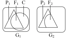
P1 F1 C
G1
P2 F2
[image:4.612.137.251.652.718.2]G2
Figure 2 Vertex Cover Refinement
4.1 Vertex Cover Based Refinement
We use a vertex cover C to refine a matching M. A vertex cover C of a graph G is a subset of nodes
in V(G), that is, C⊆V(G), such that for every edge
(u,v)∈E(G),we have u∈C or v∈C. A minimum
vertex cover of graph G is a vertex cover with the minimum number of nodes.
A vertex cover C of G is a minimal vertex cover, if there does not exist a vertex cover C’ of G such
that C’⊂C.
A set of nodes C is a vertex cover of graph G if and only if its complement I =V(G)−C is an independent set of G. Here, an independent set I of G is a subset of nodes in V(G), that is, I⊆V(G),
such that for any u∈I and v∈I, (u,v)
∉
E(G).Below, we introduce some notations we use to refine a matching M based on vertex cover. Suppose we match two graphs G1 and G2, and M is a matching found. Let P1 and P2 be the matched nodes in G1 and G2, respectively, using the
matching M. For any (u,v)∈M,wehave u∈P1 and
v∈ P2. Given a cover C of G1, we use F1 to denote
C∩P1.
For any subset of nodes S⊆P1, we use M[S] to
denote the corresponding matched part of S in P2
using matching M. For any subset of nodes S⊆P2,
we use M−1[S] to denote the matched part of S in P1 using matching M. Let F2=M[F1]. The relationships among G1,G2,P1,P2,F1,F2 and C are illustrated in Figure. 2
The vertex cover structure plays an important role when wematch two graphs G1 and G2. It allows us to focus on one graphG1, with the assistance of its vertex cover. The intuition is as follows. By definition, a vertex cover of G1 is the set of nodes that covers all possible edges in G1. This implies that a node in the vertex cover can possibly have many edges to cover (or possibly have many matched edges with another graph G2). A vertex cover C of G1 divides V(G1) into three
parts, F1= C∩P1, C−F1 and V(G1)−C. The
4.2 Refinement And Its Optimality
Given two graphs G1 and G2, a matching M, and
a vertex cover C of G1, we give a refinement M+(C)
of M, and show its optimality below.
First, we show how to obtain a refinement M+(C)
of M. We build a complete weighted bipartite graph Gb. On one side, Gb includes the nodes in V(G1)−C, and on the other side, Gb includes the
nodes in V(G2)−F2. For any node u∈V(G1)−C and
node v∈V(G2)−F2, we add an edge (u,v) in E(Gb),
and the weight of the edge (u,v) is defined as follows.
w(u,v) =|M[N(u)∩F1]∩(N(v)∩F2)| (2)
where N(u) and N(v) are the sets of immediate neighbors of u and v in graphs G1 and G2, respectively. Intuitively, w(u,v) is the contribution of the matched edges if we match u in graphG1 with v in graph G2. Next, we find the maximum weighted bipartite matching Mb of Gb using the Hungarian algorithm, such that the total weight of edges in Mb is maximized. We obtain our new
matching M+(C) as follows.
M+(C) = (M∩(F1×F2))∪Mb (3)
where F1×F2 is the cartesian product of F1 and
F2. It includes all pairs (u,v) such that u∈F1 and v
∈F2.
Example 1 To make it simpler, let’s only consider part of the matching in the initial matching. Suppose the first graph in figure 3(a) is the partial graph induced by nodes {u6, u8, u11, u12, u13} in G1, and the second graph in figure 3(b)
is the partial graph induced by nodes
{v6,v8,v11,v12,v13} in G2. In the initial matching M generated in Example 4, only three edges are matched, which is showed as the bold edges in figure 3(a)(b). We have P1={u6, u8, u11, u12, u13} and P2={v6,v8,v11,v12,v13}. Suppose C={u6, u8,
u12},we have F1=C∩P1={u6, u8, u12} and
F2=M[F1]={v6,v8,v12}. In the bipartite graph Gb, the left part consists of the nodes in V(G1)−C, which is {u11, u13}, and the right part consists of the nodes in V(G2)−F2, which is {v11,v13}. The graph Gb is shown in figure 3(c). For the edge (u11,v11), its weight is 2 because if we match node u11 with node v11, 2 edges will be matched in the original graphs, that is, edge (u11, u8) is matched to edge (v11,v8), and edge (u11, u12) is matched to edge (v11,v12). The maximum weighted bipartite matching of Gb is Mb ={(u11,v11), (u13,v13)}. Modifying the result in Example 1 using the new matching, we can improve the number of matched edges from 18 to 20. Similarly, we can refine matching pairs {(u2,v7), (u7,v2)} to be {(u2,v2), (u7,v7)} such that it will improve the number of
matched edges to 21, which is the optimal value in this example.
u
6
u11
u13 u12
u8
(a) (b)
(c) (d)
Figure 3 Vertex Cover Refinement Example. (A) G1, (B) G2, (C) C ={U6, U8, U12},
(D) C ={U11, U12, U13}
Second, we give the optimality of M+(C) over a
matching space M. The space M is a set of matching between nodes in G1 and G2, such that
for any matching M’, M’∈M if and only if M’∩
(F1×F2)=M∩(F1×F2) and M’((C−F1)×V(G2)) =
∅ . For the matching M, a matching M’∈M, if and
only if the matching for nodes in F1 is not changed
and the matching for nodes in C−F1 is ∅ . The
second condition can also be expressed as
M’[C−F1]=∅ .
[image:5.612.328.496.119.294.2]Theorem 1 Suppose min = min{|V(G1)|−|C|,
|V(G2)|−|F2|} and max = max{|V(G1)|−|C|,
|V(G2)|−|F2|}, then we have:
(1) |M|=
min
0
min! max!
and
! (min )! (max )!
i= i i i
×
× − × −
∑
min
max!
| | (max 1)
(max-min)!≤M ≤ +
(2) M ∈M
(3) M+(C) ∈M and
(4) M+(C) is optimal in M
Proof 1 We prove it step by step.
(1) To make things simple and without loss of
generality, we assume |V(G1)|−|C|≤|V(G2)|−|F2|,
then min =|V(G1)|−|C| and max =|V(G2)|−|F2|. Since V(G1)−C and V(G2)− F2 are the included parts of G1 and G2, respectively, we only consider the number of different matching between V(G1) − C and V(G2) − F2. Suppose in V(G1)−C, there are i nodes that participate in the matching in M, there are min
i
C different selections of the i nodes, and for
each selection, there are max
i
P different matching
between the i nodes and nodes in V(G2)−F2. There
are totally min
i
C × max
i
P different matching for a
|M|= min
min max 0
i i i
C P
= ×
∑
min 0min! max! ! (min )! (max )!
i= i i i
× =
× − × −
∑
When i= min, we have:
min max
max! | |
(max-min)!
i i
M≥C ×P =
If we remove the constraint that different nodes in V(G1)−C must match different nodes in V(G2)−F2, each node in V(G1)−C will have max + 1 choices include max nodes in V(G2)−F2 and an empty match. The number of different relaxed matching is then changed to (max+1) min which is an upper bound of |M|.
(2) We only need to prove that M satisfies the two conditions of M. For the first condition,
obviously, M∩(F1×F2)=M∩(F1×F2). For the
second condition, the part C−F1 is the nodes in C
that are not matched in M, so M[C−F1] =∅. As a
result, M∩((C−F1)×V(G2)) =∅.
(3) We need show that M+(C) satisfies the two
conditions of M.
– For the first condition, we have:
M+(C)∩(F1×F2)
= ((M∩(F1×F2)) Mb)∪ ∩(F1×F2)
= (M∩(F1×F2)) (Mb∪ ∩(F1×F2))
Since Mb only includes nodes in V(G1)−C and
V(G2)−F2,wehave Mb∩(F1×F2) =∅.As a result,
M+(C)∩(F1×F2)=M∩(F1×F2).
– For the second condition, we have:
M+(C)∩((C−F1)×V(G2))
= ((M∩(F1×F2))∪ Mb)∩((C−F1)×V(G2))
=
((M∩(F1×F2))∩((C−F1)×V(G2)))∪(Mb∩((C−F1)×
V(G2)))
Moreover, we have
(M∩(F1×F2))∩((C−F1)×V(G2)) =∅, because
M∩((C−F1)×V(G2)) =∅ is already proved in (2)
and Mb∩((C−F1)×V(G2)) =∅ due to the fact that
Mb does not contain any nodes in C−F1. Thus, we
have M+(C)∩((C−F1)×V(G2)) =∅.
(4) For any matching M’∈M, we define a
matching Mb' as
'
b
M =M’∩
((V(G1)−C)×(V(G2)−F2)). We use scoreb(Mb) to
denote the total weight for the bipartite matching
Mb of the bipartite graph Gb. We claim: (a) M is a b'
bipartite matching of Gb; (b) score( Mb' ) =
scoreb(
'
b
M )+score(M∩(F1×F2)); (c) score(M+(C))
= scoreb(Mb)+score(M∩(F1×F2)).
For (a), it is obvious because of two reasons. (1) '
b
M only contains the nodes in V(G1)−C and
V(G2)−F2, which is exactly the set of nodes in Gb.
(2)Any edge in '
b
M is also an edge of Gb since Gb is a complete bipartite graph.
For (b), we have:
score(M’)= score(M’∩((C (V(G1)−C))×(F2∪ ∪
(V(G2)−F2))))= score((M’∩(C×F2)) (M’∪ ∩(C
×(V(G2)−F2)))∪(M’∩((V(G1)−C)×F2))∪(M’∩((V
(G1)−C)×(V(G2) −F2)))). Since C×F2,
C×(V(G2)−F2), (V(G1)−C)×F2 and (V(G1)−C) ×(V(G2)−F2) are mutually exclusive with each other, we have:
score(M’)= score(M’∩(C×F2))+score(M’∩(C
×(V(G2)−F2)))+score(M’∩((V(G1)−C)×
F2))+score(M’∩ ((V(G1)−C)×(V(G2)−F2)))
Since M’[F1]=F2 and M’[C−F1]=∅, we have
M’[C]=M’[F1]∪M’[C−F1]=F2, and thus M’∩(C
×(V(G2)−F2))=∅. Since M’−1[F2]=F1 and F1⊆C,
we have M’∩((V(G1)−C)×F2) =∅.
We also have:
M’∩(C×F2)= M’∩(((C−F1) F1)×F2) ∪
= (M’∩((C−F1)×F2))∪(M’∩(F1×F2))
= M’∩(F1×F2)
The last equation is due to M’∩((C−F1)×F2) =∅
because M’[C−F1]= ∅. Since M’∩(F1×F2)
=M∩(F1×F2), we can derive:
score(M’) = score(M’∩(F1×F2)) +score(M’∩
((V(G1)−C)×(V(G2)−F2)))
= score(M∩(F1×F2)) + score( '
b
M )
We only need to prove score(M ) = scoreb' b(
'
b
M ). Since V(G1)−C is a independent set which only have edges with C and C is the excluded part of the
matching M’ ,we can derive that
score(M’∩((V(G1)−C)× (V(G2)−F2))) only
consists of the contributions of the edges
(u,v)∈E(G1) such that u∈C and v V(G1)−C. ∈
From the construction of Gb, the contribution for
each v∈V(G1)−C in M’ is just the weight (v, M’[v])
in the bipartite graph Gb.
This implies score( '
b
M ) = scoreb(
'
b
M ).
For (c), it can be easily derived from (b) because
M+(C) ∈Mand Mb = M+(C) ∩ ((V(G1)−C)×(V(G2)
− F2)).
Since Mb is the maximum weight bipartite
matching of Gb, we have costb(Mb) ≥ costb(
M
b' ).Hence, we have:
score(M+(C)) =score
b(Mb) +score(M∩(F1×F2))
≥scoreb( '
b
M )+score(M∩ (F1×F2))= score(M’) As a result, M+(C) is the optimal solution in M. The theorem holds.
Theorem 1 shows that the size of M is
exponentially large. Both M and M+(C) are
elements in M, and M+(C) is the optimal matching
for all matching in M. It implies that M+(C) is the
best among a large number of matching in M and
score(M+(C)) ≥ score(M). For two graphs with
cover can be assumed as 1,000 (50%) reasonably.
M+(C) is the best among a factorial of 1,000 (1,000!)
possible matching.
4.3 Randomly Refinement Excluding C−F1 If M itself is an optimal matching in M, or the selected vertex cover C includes most nodes in G1
that are not well matched, it is possible that M+(C)
cannot improve M. As an example, suppose C ={u11, u12, u13}, in Example 1, then the new bipartite graph Gb is the one shown in Figure 3(d). In other words, using the maximum weighted
bipartite matching of Gb, the matching M+(C)
might be the same with M. The reason is that the mismatched nodes are excluded by the vertex cover C to refine. We give an approach based on two strategies to solve such a problem. (1) Making C smaller, such that more mismatched nodes can be included and thus can be used to refine. (2) Iteratively refining the current matching using different vertex covers, such that every mismatched node will have a chance to be included to refine. The first strategy is based on the following Lemma.
Lemma 1 For any two vertex covers C1 and C2
of G1, if C1 ⊆ C2, then score(M+(C1)) ≥
score(M+(C2)).
Proof 2 Suppose M(C1) and M(C2) are the matching spaces generated by C1 and C2, respectively. We use F1(C1), F1(C2), F2(C1), and F2(C2) to denote F1 generated by C1, F1 generated by C2, F2 generated by C1, and F2 generated by
C2, respectively. Since we have F1(C1) ⊆ F1(C2)
and F2(C1) ⊆ F2(C2), we need show M(C2) ⊆
M(C1). For any M’∈M(C2), we have:
M’∩(F1(C2)×F2(C2))=M∩(F1(C2)×F2(C2)),
M’∩((C2−F1(C2))×V(G2))= ∅. Since
F1(C1)×F2(C1)⊆F1(C2)×F2(C2), we derive: M’∩
(F1(C1)×F2(C1))=M∩(F1(C1)×F2(C1)). We also
have C1−F1(C1)⊆C2−F1(C2), which yields: M’∩
((C1−F1(C))×V(G2))= ∅. Thus, we have M’∈
M(C1), that is, M(C2)⊆M(C1). Since M+(C1) and
M+(C2) are the optimal solutions in M(C1) and
M(C2) respectively, we have score(M+(C1))≥
score(M+(C2)).
In order to make C small, a straight forward way is to find a minimum vertex cover of G1. This method is not practical for two reasons. (1) Finding a minimum vertex cover of a graph is NP-hard. (2) In a minimum vertex cover, the mismatched nodes do not have a chance to be included to refine. To avoid these, we use a minimal vertex cover instead, because (1) a minimal vertex cover is easy to be found and (2) the number of different minimal vertex covers for a graph is much larger than the
number of different minimum vertex covers. Thus, a minimal vertex cover gives the mismatched nodes in a minimum vertex cover more chances to be refined.
Algorithm 2 select-random-cover (G) Require: agraph G;
Ensure: a randomly selected minimal cover of G;
1: L ←shuffled nodes in V (G); C ←∅;
2: for all u ∈ L do
3: if
∃
(u,v)∈E(G), s.t. v∉
C then C ←C ∪{u};4: for all u ∈ C do
5: if C−{u} is a vertex cover of G then C←C
−{u}; 6: return C;
The approach to randomly select a minimal vertex cover of graph G is shown in Algorithm5. First, in line1, we shuffle all nodes in the graph and put them into a list L, such that any permutation of V(G) has the same probability in L. In lines 2–3, we find a vertex cover of G by adding node in L one by one. For any node to be added, we add it into the vertex cover if and only if it contributes at least one edge to the currently covered edges (line 3). This operation can be implemented as follows. For every node in the graph, we maintain its number of uncovered edges, which is initially set to be the degree of the corresponding node. Every time before we add a new node into the cover, we first check its number of uncovered edges. If it is 0, we skip the node, and continue to add the next one in L. Otherwise, we add the node into the cover, and traverse its adjacent nodes in the graph. For each adjacent node, we decrease its number of uncovered edges by 1. In such a way, the total complexity for line 2–3 is O(|E(G)|), since every edge in G is visited at most once. Lines 4–5 make the current vertex cover minimal by removing those useless nodes, such that the removal of such nodes does not influence any edge currently covered. The following lemma shows that, for any minimal cover C of a graph G, there are considerable number of ways for Algorithm 2 to generate C.
Lemma 2 For any minimal vertex cover C of graph G, there are at least |C|!×|V(G)−C|! permutations of V(G),such that Algorithm 2 generates C.
conditions in line 3 are all unsatisfied because C is already a vertex cover of G. So after the loop in lines 2-3, C is generated. Since C is already minimal, the loop in lines 4–5 will eliminate no node. Thus, Algorithm 2 can generate C.
Algorithm 3 refine (G1, G2, M)
Require: two graphs G1 and G2, and the matching M;
Ensure: a refined matching M;
1: while M is updated or it is the first iteration do 2: for i = 1 to X do
3: G ←random selection between G1 and G2;
4: C ←select-random-cover (G);
5: compute M+(C);
6: if score(M+(C)) > score(M) then M ← M+(C);
7: return M;
The main refine approach is an iterative algorithm shown in Algorithm 3. We iteratively update the current matching until the matching is not improved in a certain iteration. In each iteration (lines 2–6), we try X times to find a new random minimal vertex cover C (line 4), generate the
matching M+(C) using the method introduced above
(line 5), and update the current matching if M+(C) is
a better matching (line 6). Here, X is a constant (≥ 1)
in order to avoid selecting a bad cover to terminate the whole process. In our experiments, when X = 5 and X = 10 over 92 and 99% of the nodes have a chance to be included to refine. We use X = 5. Note that in line 3, we choose C to be a vertex cover of either G1 or G2 with the same probability to increase the randomness.
Algorithm 4 refine (G1, G2, M)
Require: two graphs G1 and G2, and the matching M;
Ensure: a refined matching M;
1: while M is updated or it is the first iteration do 2: for i = 1 to X do
3: GF ←random selection between G1[P1] and
G2[P2];
4: F ←select-random-cover (GF );
5: compute M*(F);
6: if score(M*(F)) > score(M) then M ← M*(F);
7: return M;
Theorem 2 The time complexity of Algorithm 4 is O(m· n3), for m = min{|E(G1)|, |E(G2)|} and n = max{|V(G1)|, |V(G2)|}.
Proof 4 Algorithm 4 is the main refinement. The while loop in line 1 will repeat for at most m times because the optimal solution can match at most m edges and in each loop, the number of edges for the latest solution will be increased for at least 1. In each loop, the dominant part is finding the maximum weight bipartite matching using the
Hungarian algorithm which can be done in O(n3).
Since X is a constant, the total time complexity for
Algorithm 4 is O(m · n3).
Theorem 2 shows an upper bound of the time complexity for Algorithm 4. In practice, the processing time for the algorithm is much smaller than the upper bound because the initial matching M has already matched a lot of edges. In the case when m and n are large, Algorithm 4 can be very slow. We discuss two approaches to make Algorithm6 faster, with possible loss of matched edges. The goal is the same as before to match as many edges as possible. The first approach is to stop the iteration when the algorithm converges
slowly, that is, no larger than δ new matched edges
are found in a certain iteration. In such away, them part in the time complexity can be largely reduced. The second approach is to enlarge the size of the vertex cover, for example, adding some nodes with the minimum number of unmatched edges into the current vertex cover. The bipartite matching is only conducted on the nodes that are not in the vertex cover. If the size of the vertex cover increases, the number of nodes used in the bipartite matching decreases, thus the time used for matching nodes decreases. In such a way, the n3 part in the time complexity can be reduced.
4.4 Randomly Refinement Including C−F1
In this section, we show that M+(C) can be
further improved. Recall that in our previous
approach to compute M+(C), the nodes in C−F1 of
G1 are excluded to refine. In order to refine the nodes in C−F1, we build a new weighted bipartite
graph *
b
G as follows. On one side, *
b
G includes all
nodes in V(G1)−F1, and on the other side, Gb*
includes all nodes in V(G2)−F2. For any node v ∈
V(G1)−F1 and node u∈V(G2)−F2, there is an edge
(u,v)∈E *
b
G ) with weight defined in Eq. (6).
Suppose the maximum weighted bipartite matching of Gb*is
*
b
M , the new matching M*(F1) is defined as
follows.
M*(F1)=(M∩(F1×F2))∪ *
b
M (3)
We now define a matching space M*. For any
matching M’ between graphs G1 and G2, M’∈M*
if and only if it satisfies the following two conditions.
(1) M’∩(F1×F2)=M∩(F1×F2)
(2)F1∪(V(G1)−P1−M’−1[V(G2)−P2]) is a vertex
cover of G1.
Theorem 3 M⊆M* and suppose M∗
M is the
optimal solution among all matching in M∗, we
have score(M*(F1))≥score(M∗
Proof 5 For ∀M’∈M, we have
M’∩(F1×F2)=M∩(F1×F2) and M’[C−F1]= ∅. The
first condition is the same as the first condition of
M*. Since M’[C− F1]= ∅,
we have (C−F1)∩M’−1[V(G2) − P2]=
∅. We also
have (C−F1) M’∪ −1 [V(G2)−P2] ⊆ V(G1)−P1,
accordingly, C−F1⊆V(G1)−P1−M’−1[V(G2)−P2],
and thus C⊆F1∪(V(G1)−P1−M’−1 [V(G2)−P2]).
Since C is a vertex cover of G1,
F1∪(V(G1)−P1−M’−1[V(G2)−P2]) is a vertex cover
of G1, hence we have M’∈M*. Thus M⊆M* holds.
We now prove that score(M*(F1)) ≥ score(M∗
M).
Suppose C*=F1∪(V(G1)−P1− M∗
M-1[V(G2)− P2]),
we know C* is a vertex cover of G1. Since M∗
M
[V(G1)−P1] ⊆V(G2) − P2, we have:
M∗
M[C*−F1]=
M∗
M [V(G1)−P1−M∗M-1[V(G2)−P2]]= ∅.Thus, we
have M∗
M∈M using vertex cover C*, which implies
(see the proof of Theorem 4):
score(M∗
M) = score(M∩(F1×F2))+scoreb(Mb)
where Mb is the maximum weight bipartite matching of Gb generated by C*. We also have
score(M*(F1)) ≥score(M ∩ (F1 × F2)) +
scoreb( *
b
M ). Since Gb⊆ *
b
G , we have:
score(M*(F1))≥score(M∩(F1×F2)) + scoreb( *
b M )
≥score(M∩(F1×F2))+scoreb(Mb)= score(M∗M).
We last prove score(M∗
M)≥score(M+(C)). This
can be derived directly from M⊆M* since M∗
M is
optimal in M* and M+(C) is optimal in M.
Theorem 3 implies that the new space M* is larger than the space M in refinement excluding C−F1, and the new matching M*(F1) is no worse than the optimal matching in M*. This implies that
score(M*(F1)) ≥ score(M+(C)), where M+(C) is the
optimal matching in M. It is worth noticing that the cover C of G1 does not participate in the construction of M*(F1) directly. The matching M*(F1) can be computed as long as F1 is generated, and F1 can be computed easily by the following lemma.
Lemma 4 Suppose G1[P1] is the subgraph of G1 induced by P1. If C is a vertex cover of G1, then C∩P1 is a vertex cover of G1[P1], and if CP1 is a vertex cover of G1[P1], then there exists a vertex
cover C of G1 such that CP1⊆ C.
Proof 6 We first prove that if C is a vertex cover
of G1, then C∩P1 is a vertex cover of G1[P1].
Suppose C∩P1 is not a vertex cover of G1[P1],
then there exists an edge (u,v)∈E(G1[P1]) such that
u
∉
C∩P1 and v∉
C∩P1. Note that C is a vertexcover of G1,wehave u∈C or v C. Without loss of ∈
generality, we suppose u∈C. Since u
∉
C∩P1, wehave u∈C−(C∩P1),which contradicts with
u∈V(G1[P1]). Thus, C∩P1 is a vertex cover of
G1[P1].
We then prove that if CP1 is a vertex cover of G1[P1], then there exists a vertex cover C of G1
such that CP1⊆C. We only need to prove that
C=CP1∪(V(G1)−P1) is a vertex cover of G1. For
any (u,v)∈E(G1), if u P1 and v P1, (u,v) is ∈ ∈
covered by C because CP1 is a vertex cover of G1[P1]. Otherwise, without loss of generality, we
suppose u
∉
P1, then u∈V(G1)−P1⊆C, so (u,v) isalso covered by C. As a result, all edged in E(G1) can be covered by C, thus C is a vertex cover of G1.
Based on Lemma 1, we can derive that the vertex cover of G(P1), F1, is enough to generate M*(F1). Our new refinement algorithm is shown in Algorithm 4 which is the refine used in Algorithm 2.We use X = 5. Comparing to Algorithm 3, there are two major modifications. The first is about the cover computing in lines 3–4, instead of computing the cover of G1 (or G2 if we select G2 as the first graph in line 3), we only compute the vertex cover of G1[P1] (or G2[P2]). For the second modification,
instead of computing M+(C), we compute our new
matching M*(F).
5. CONCLUSION
The initial matching M is computed using the heuristics that match the anchors first followed by matching the nodes around the anchors in a top-down fashion. The heuristics used cannot guarantee that all the anchors are correctly matched. In this paper, we propose a new approach to refine the initial matching M. It is important to note that our strategy is to refine the initial matching and is not to find a completely new matching. By refinement, we mean the following two things. First, we are not to explore all possibilities without a goal when we refine a matching. In other words, we refine a matching M to a better one which is most likely to exist and can be identified. Second, we consider the efficiency when refining a matching. In our approach, each time we focus on a subset of nodes to refine by excluding a subset of nodes and including a subset of nodes. The set of nodes to be excluded from refinement at one time is neither large nor small. Also, we give every node in the graphs a chance to be refined.
be refined. We show the optimality of our refinement. We also show how to randomly refine
matching with different combinations. Our
refinement can improve the matching quality with small overhead for both unlabeled and labeled graphs.
REFERENCES:
[1] T. Plantenga, “Inexact subgraph isomorphism in
MapReduce”, Journal of Parallel and
Distributed Computing, Vol. 73, No. 2, 2013, pp. 164-175.
[2] F. Kuhn, and M. Mastrolilli, “Vertex cover in graphs with locally few colors”, Information and Computation, Vol. 222, No. 0, 2013, pp. 265-277.
[3] A. Egozi, Y. Keller, and H. Guterman, “A Probabilistic Approach to Spectral Graph Matching”, Pattern Analysis and Machine Intelligence, IEEE Transactions on, Vol. 35, No. 1, 2013, pp. 18-27.
[4] T. S. Caetano, J. J. McAuley, C. Li et al., “Learning Graph Matching”, Pattern Analysis and Machine Intelligence, IEEE Transactions on, Vol. 31, No. 6, 2009, pp. 1048-1058 [5] L. Zhi-Yong, Q. Hong, and X. Lei, “An
Extended Path Following Algorithm for Graph-Matching Problem”, Pattern Analysis and Machine Intelligence, IEEE Transactions on, Vol. 34, No. 7, 2012, pp. 1451-1456.
[6] H. Xiong, D. Xiong, Q. Zhu et al., “A Structured Learning-Based Graph Matching Method For Tracking Dynamic Multiple Objects”, Circuits and Systems for Video Technology, IEEE Transactions on, Vol. PP, No. 99, 2012, pp. 1-1.
[7] P. Doshi, R. Kolli, and C. Thomas, “Inexact matching of ontology graphs using
expectation-maximization”, Web Semantics: Science,
Services and Agents on the World Wide Web, Vol. 7, No. 2, 2009, pp. 90-106.
[8] T. Ersal, H. K. Fathy, and J. L. Stein, “Structural simplification of modular bond-graph models based on junction inactivity”, Simulation Modelling Practice and Theory, Vol. 17, No. 1, 2009, pp. 175-196.
[9] Z. Nutov, “Survivable network activation problems”, Theoretical Computer Science, No. 0, 2012.
[10] S. Kpodjedo, P. Galinier, and G. Antoniol, “Using local similarity measures to efficiently address approximate graph matching”, Discrete Applied Mathematics, No. 0, 2012.
[11] L. Sun, and T. Chen, “Comparing the Zagreb indices for graphs with small difference between the maximum and minimum degrees”, Discrete Applied Mathematics, Vol. 157, No. 7, 2009, pp. 1650-1654.
[12] J.-K. Hao, and Q. Wu, “ Improving the
extraction and expansion method for large
graph coloring ” , Discrete Applied
Mathematics, Vol. 160, No. 16, 2012, pp. 2397-2407.
[13] A. Bhattacharjee, and H. Jamil, “WSM: a novel algorithm for subgraph matching in large weighted graphs”, Journal of Intelligent Information Systems, Vol. 38, No. 3, 2012, pp. 767-784.
[14] M. Zaslavskiy, F. Bach, and J. P. Vert, “A Path Following Algorithm for the Graph Matching Problem”, Pattern Analysis and Machine Intelligence, IEEE Transactions on, Vol. 31, No. 12, 2009, pp. 2227-2242.
[15] L. Zhu, W. Keong Ng, and J. Cheng, “Structure and attribute index for approximate graph matching in large graphs”, Information Systems, Vol. 36, No. 6, 2011, pp. 958-972.
[16] T. Yamada, and T. Shoudai, “Efficient Pattern Matching on Graph Patterns of Bounded Treewidth”, Electronic Notes in Discrete Mathematics, Vol. 37, No. 0, 2011, pp. 117-122.
[17] J. Lebrun, P.-H. Gosselin, and S. Philipp-Foliguet, “Inexact graph matching based on kernels for object retrieval in image databases”, Image and Vision Computing, Vol. 29, No. 11, 2011, pp. 716-729.
[18] C. Jiefeng, J. X. Yu, and P. S. Yu, “Graph Pattern Matching: A Join/Semijoin Approach”, Knowledge and Data Engineering, IEEE Transactions on, Vol. 23, No. 7, 2011, pp. 1006-1021.
[19] R. Erman, M. Krnc et al., “Improved induced
matching in sparse graphs”, Discrete Applied
Mathematics, Vol. 158, No. 18, 2011, pp. 1994-2003.
[20] D. Emms, R. C. Wilson, and E. R. Hancock, "Graph matching using the interference of discrete-time quantum walks," 7th IAPR-TC15 Workshop on Graph-based Representations (GbR 2007), 2009, pp. 934-949.
![figure 3(a)(b). We have P1={u6, u8, u11, u12, u13} and P2={v6,v8,v11,v12,v13}. Suppose C={u6, u8, u12},we have F1=C ∩ P1={u6, u8, u12} and F2=M[F1]={v6,v8,v12}](https://thumb-us.123doks.com/thumbv2/123dok_us/8916284.961978/5.612.328.496.119.294/figure-p-suppose-c-f-p-f-m.webp)
