EXTENDING TEMPORALLY ER MODEL FOR DESIGNING
TEMPORAL DATABASES WITH MULTIPLE TIME
GRANULARITIES
CHUNLONG YAO,FENGLONG FAN, LAN SHEN, XU LI
School of Information Science and Engineering, Dalian Polytechnic University,
Dalian 116034, P.R. China
E-mail: [email protected]
ABSTRACT
Abstract Entity-Relation (ER) model may be used for different but related purposes, e.g. to model real world for analysis, to describe a database scheme of a computer system for design. In recent years, with the increasing needs of time-related application, how to extend the ER model to enable it to properly capture time-varying information has been active area of research. By extending temporally traditional ER models, we propose a new temporal ER model, which is called ETER model. For the ETER model, we introduce two new constructs including variety granularity and time cardinality. We discuss how to specify time-varying attributes and relationships using these constructs, and how to specify TFDs constraints. Therefore, the ETER model and temporal normalization theory can be integrated to design temporal databases with multiple time granularities.
Keywords: ER Model, temporal database, database design, temporal functional dependency (TFD)
1. INTRODUCTION
We know that there are two approaches to implement a temporal database system. One is that built-in temporal support is offered by a DBMS [1], and the DBMS need to be extended temporally. Another one is that a temporal middleware [2] is used between user application and DBMS to accept requests of the temporal applications, and map temporal SQL statements to regular SQL statements. These two approaches are based on relational model in general. As a result, our objective is seeking methodology of logical design for temporal databases based on the relational model. Similar to methodology of logical design using ER model for relational databases (e.g. see [3]), we may design temporal databases with multiple time granularities using temporal ER models. For this purpose, the temporal ER model used can support for multiple time granularities, and specifies temporal data dependencies constraints, and be mapped to an appropriate temporal data model.
At present, a few decades temporal data models based on the relational model have proposed (e.g. see [4] [5]). The concept of temporal module schemes [6] is rather general, and the results and concepts related to the temporal module scheme are
readily translated in terms of other temporal data models. Temporal module schemes [6] provide a unified interface for accessing different temporal information systems. For normalizing temporal databases, a few temporal data dependency was proposed (e.g. see [6] [7]). Based on temporal functional dependencies (TFDs), the systemic theory of normalization is discussed for temporal databases with multiple time granularities, and the advantages using TFDs to express temporal data constraints and to design temporal databases are introduced by comparing with some other temporal data dependencies [6]. So it is a good choice to use TFDs to design temporal databases with multiple time granularities in terms of temporal module schemes.
TID TEACHER Address Name
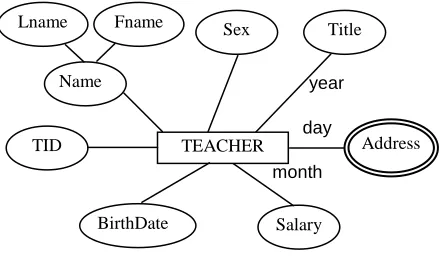
Figure 1: An Example Of Attributes
Lname Fname Sex Title
Salary BirthDate
year
day
month
development of temporal ER models. At present, many temporal ER models, e.g. TERM [9], MOTAR [10], TERC+ [11], HDRM [12] and TimeER (see [13] [14] [15]) etc, were developed. For RFID data management, the DRER model [16] was presented by adding dynamic relationships in ER models. In recent years, some researchers explored reasoning over temporal ER models based on description logics (e.g. see [17] [18]). In a temporal ER model, support for the specification of advanced temporal constraintswould be desirable [19]. According to the best author’s knowledge, existing temporal ER models do not consider that entities may be variable with different granularities relative to the other entities in relationships, and how to specify TFDs with multiple time granularities.
By extending temporally traditional ER models, we propose a new temporal ER model, which is called ETER model. Our model not only can specify different time granularities for attributes but also for entities in relationships. Besides supporting for multiple time granularities, our model can specify TFDs constraints and can be converted into temporal module schemes..
2. COMPONENTS OF THE ETER MODEL
An ETER model may be described visually by a diagram, which is said to be ETER diagram. Similar to traditional ER model, there exist three kinds of components including entity types, attributes and relationship types in the ETER model. We assume that the reader is familiar with the properties of the ER model and ER diagram [20], and only new properties and constructs are described. In ETER models, we use temporal types [6] to describe time granularities.
The concept of temporal type was introduced in [6], which will be shown below. We denote R the set of all real numbers, and 2R the power set of R.
Definition 1(Temporal Type). A temporal type is a mapping µ from the set of the positive integers (the time ticks) to 2R (the set of absolute time sets) such that for all positive integers i and j with i<j, the following conditions are satisfied.
1) µ(i)≠φand µ(j)≠φ imply that each real number in µ(i) is less than all real numbers in µ(j), and
2) µ(i)=φ implies µ(j)=φ.
Intuitive temporal types (e.g., day, month, week,
year) satisfy the above definition. For example, we can define a special temporal type year begin from year 1800 as follows: year (1) is the absolute time set (an interval of real) corresponding to the year 1800, year (2) is the set of absolute time set corresponding to the year 1801.
Definition 2 (Finer-Than Relation). Let µ1and µ2 be temporal types. Then µ1 is said to be finer than µ2, denoted µ1≼µ2, if for each i, there exists j such that µ1 (i) ⊆µ2 (j).
For each pair temporal types µ and ν, if µ≼ν and µ≠ν, we denote µ≺ν. By the definition, µ≼µ for
each temporal type µ, and for any pair temporal
types µ1 and µ2,if µ1≼µ2 and µ2≼µ1, then µ1 = µ2. There exists a unique least upper bound of the set of all temporal types denoted by µTop, and a unique greatest lower bound, denoted by µBottom. These top and bottom elements are defined as follows: µTop (1)=R and µTop (i)=φ for each i>1, and µBottom (i)=φ for each positive integer i. For each pair temporal types µ1 and µ2, there exist a unique least upper bound lub (µ1, µ2) and a unique greatest lower bound glb (µ1,µ2) of these two temporal types.
In the following sections in this paper, if we do not declare in advance then each temporal type used by us is the Gregorian time [21].
2.1 Attributes
Several types of attributes exist: simple attributes and composite attributes [20]. For any composite attribute CA, we denote coll (CA) the set
of all simple attributes that CA involves. For
example, for the composite attribute Name shown in Figure 1, coll (Name) = {Fname, Lname}.
For example, we view the attribute SALARY of entity type EMPLOYEE, if the salary of an employee cannot be changed in a month, then the variety granularity of SALARY is month, i.e. vg
(SALARY)=month. In the ETER, for each
attribute, its variety granularity must be designated. Attributes may be divided into non-temporal attributes and temporal attributes according to its variety granularities.
Non-temporal Attributes. For any attribute, if its variety granularity is µTop, then the attribute is non-temporal. It is the same as the traditional ER model that the value of a non-temporal attribute is invariable over time. In the ETER diagram shown in Figure 1, the attributes TID, Name, BirthDate and Sex are non-temporal attributes.
Time-Invariant Keys and Key Attributes. A time-invariant key (TIK) of an entity type is a set of non-temporal and simple attributes, such that the values of these attributes can be used to identify uniquely entities of the entity type throughout lifespan, and its any subset cannot do that. The lifespan of an entity whose information is stored in a database is the time that the entity exists in the database. It is possible that an entity type may have several time-invariant keys. In the case where several time-invariant keys exist, we usually choose a semantically meaningful time-invariant key as the primary time-invariant key (PTIK). For an entity type, we call the attributes that belong to the PTIK of the entity type key attributes. Key attributes are underlined in the ETER diagram. For example, the attribute TID is PTIK of entity type TEACHER in the ETER diagram shown in Figure 1.
Temporal Attributes. If the variety granularity of an attribute is any temporal type that is not µTop, then the attribute is temporal. The values of a temporal attribute may be changed over time. For any temporal attribute TA whose variety granularity is µTop, semantics may be expressed as follows.
1) If TA is a single-valued attribute, then the attribute TA has unique value in any time tick of µ;
2) If TA is a multi-valued attribute, then TA may have a group of values at a given time instant, and it has unique a group of values in any time tick of µ.
For each temporal attribute, its variety granularity is explicitly labeled on the straight line linking it and its entity type or relationship type in the ETER diagram. As shown in Figure 1, the attributes Title, Salary and Address are temporal attributes of entity type TEACHER. From the diagram, we know that each teacher has unique title
in a year; each teacher has unique salary in a month; each teacher may have different addresses at given time instant, and these addresses cannot be changed in a day.
2.2 Relationship Types
A relationship is an abstract expression of semantic relations within a thing or among things. For example, a specific student studies a specific course, as show a relationship between a student entity and a course entity. A relationship type R of degree n is a n-tuple <E1, E2, …, En> where each Ei (i=1, 2, …, n) is an entity type. Each relationship
in R is an n-tuple r = <e1, e2, …, en> where each ei ∈ Ei (i=1, 2, …, n).
2.2.1 Time Cardinalities
Generally, for a relationship type R = < E1, E2, …,
En >, each Ei (i=1, 2, …, n) may be associated with
a time cardinality <µ, ∆> where µ is a temporal type, and ∆ is a positive integer 1 or m, n, p etc representing any integer greater than 1, and the <µ,
∆> is said to be the time cardinality of Ei with respect to R, denoted by tcard (Ei, R). The
semantics of the time cardinality tcard (Ei, R) = <µ, ∆> are:
1) If ∆ = 1, then for each ej ∈ Ej (j=1, 2, i-1, i+1, …, n) , only one entity of Ei is related to it in
any time tick ofµ;
2) If ∆ = m, m or p etc representing any integer greater than 1, then for each ej ∈Ej (j=1, 2, i-1, i+1, …, n) , many entities of Ei may be related to it
at a given time instant, and unique a group of
entities of Ei are related toej in any time tick ofµ.
Definition 4 (Temporal Time Cardinality). For any time cardinality <µ, ∆>, if µ≠µTop then <µ, ∆> is said to be temporal, else <µ, ∆> is said to be non-temporal.
Obviously, the constraints expressed by non-temporal time cardinalities are the same as ones expressed by cardinalities in the traditional ER model. Let R = <E1, E2, …, En > be any
relationship type, and for each Ei (i=1, 2, …, n), tcard (Ei, R) = <µi, ∆ i>. In the ETER diagram,
usually <µi, ∆ i> is labeled on the straight line
linking Ei and R, and µi may be omitted when µi
=µTop (i.e. <µi, ∆ i>is non-temporal).
Definition 5(Relative Variety Granularity).
For an entity type E and the relationship type R that
da y
SHOP SELL COMMODITY
SID
Sname
CID Cnam
[image:4.612.86.297.407.507.2]<day, n> <day, m>
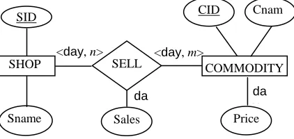
Figure 2: An example for describing time-varying information
Price Sales
da y
the relative variety granularity of E withrespect to
R.
For any relationship type, if it is necessary to keep track of the history of entities of an entity type participating the relationship type then the time cardinality of the entity type should be temporal, and the corresponding relative variety granularity selected should reflect the minimal interval of changing these entities. It is easy to describe time-varying information using time cardinalities and variety granularities. Regarding the ETER diagram shown in Figure 2 as the example, a shop need keep track of what commodities it sells and the price of each commodity everyday and daily sales of each commodity; it need keep track of each commodity is sold in which shops everyday. So for the
relationship type SELL, let tcard (COMMODITY,
SELL) = <day, m>, tcard (SHOP, SELL) = <day,
m> and vg (Sales) = day; similarly, for entity type COMMODITY, let vg (Price) = day.
Definition 6 (Temporal Relationship Type).
For a relationship type R, if there exists entity type
E participating in it, such that the time cardinality of E with respect to R is temporal then R is said to be temporal, else R is said to be non-temporal.
For example, the relationship type Sell (see Figure 2) is a temporal relationship type.
2.2.2 Weak Entity Types
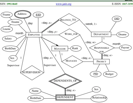
For any identifying relationship type of a weak entity type [20], the time cardinalities of owner entity types related to the weak entity type must be <µTop, 1> because for each entity of the weak entity type, owner entities related to it cannot be changed throughout its lifespan; any time cardinality may be associated to the weak entity type. For example (see Figure 3), time cardinality of the weak entity type DEPENDENT with the identifying relationship type DEPENDENTS_OF is <day, n>, which is used to keep track of the history of dependents of
each employee. This show that each employee may have many dependents at given time instant, and these dependents cannot be changed in a day.
Though a weak entity type does not have any TIK composed of its own attributes, it has the TIKs composed of the TIKs of owner entity types related to it and its partial TIKs.
2.2.3 IS-A Relationship Types
An IS-A relationship type [20] is represented by arrow flowing from the supertype to the subtype in an ETER diagram. For example, for the entity types EMPLOYEE and MANAGER shown in Figure 3, a manager is an employee too. Obviously, the entity type MANAGER is subtype of the entity type EMPLOYEE. Note that time cardinalities are not required for IS-A relationship types.
Example 1. We describe a company divided into different departments as follows: each department is in charge of a number of projects; a department keeps track of the history of projects that it is responsible for and the monthly payout of each project; each project has a manager and some employees working on the project, and a manager may manages many project at one time; each project is associated with a department that is responsible for the project; employees belong to a single department; for each employee, the company keeps track of the history of his (her) dependents; for each supervisor employee, the company keeps track of the history of supervisees who he (she) supervises; the departments would like to keep records of the histories of salary of different employee and variety of employees working for the departments; the company keeps track of what department each employee works for at what time; employees may work on many projects at one time; the company keeps track of who work on what project at what time. An ETER diagram describing the company is shown in Figure 3.
3. SPECIFYING TFDS CONSTRAINTS
Similar to traditional FDs, in order to design efficiently a temporal database scheme, temporal functional dependencies with multiple time granularities are introduced based on the temporal module and temporal module scheme [6]. The below is an example of the temporal module scheme.
Example 2. (Emp, day) is a temporal module scheme, where Emp={E# (employee number),
Ename (employee name), Salary, Dept
Similar to traditional FDs, the TFDs are very important to design temporal database schemes. In order to illustrate the TFDs constraints, we specify the semantics for the temporal module scheme (Emp, day) shown in example 2 as follows: (1) each employee has unique name, and the name is invariant over time; (2) each employee acquires unique salary in a month; (3) an employee can only work for a department in a week. Thus the temporal module scheme (Emp, day) satisfies the TFDs as follows: E# →µTop Ename; E# →month Salary; E#
→week Dept
For the ETER model, we expect to specify TFDs constraints by using time cardinalities and variety granularities. In fact, 1:1, 1:n relationship types and single-valued attributes in a ETER model can express the TFDs constraints. For example, for the ETER model shown in Figure 2, the single-valued attributes Sales and Price express the semantics as follows: each commodity that a shop sells has unique daily sales everyday; a commodity has unique price everyday. So the TFDs generated
include as follows: {SID, CID}→day Sales;
CID→day Price. As shown in Figure 3, the 1:n
relationship type BELONGS_TO expresses the semantic as follows: each employee only belongs to
a department in a week. So we may generate the TFD: EID →week DID.
For describing conveniently, we give two manipulations: for any entity type E, ptik (E) return the PTIK of E; tik (E) return a set of TIKs of E, and
ptik (E) belongs to tik (E). For any given ETER model, we may specify TFDs constraints according to the rules as follows:
C1. For each entity type E, for each simple and single-valued attribute A of E, the TFD ptik (E) →vg
(A) A is specified; for each composite and single-valued attribute C of E, the TFD ptik (E) →vg (C)
coll (C) is specified.
C2. For each relationship type R = <E1, E2,…,
En >, for each simple and single-valued attribute A
of R, the TFD ptik (E1)∪ptik (E2)∪…∪ptik (En) → vg (A) A is specified; for each composite and single-valued attribute C of R, the TFD ptik (E1)∪
ptik (E2)∪…∪ptik (En) → vg (C) coll (C) is specified.
C3. For each relationship type R = <E1, E2,…,
En > but IS-A relationship types, for each Ei (i = 1,
2,…, n), if tcard (Ei, R) = <µ, 1> then the TFD ptik BELONGS_TO
<day, n> Ename
[image:5.612.93.521.69.399.2]Address
Figure 3: An ETER Diagram For A Company
1
Supervisor
<day, n>
Supervisee
<day, n>
<day, n> <week, 1>
<day, m> EMPLOYEE
MANAGER
PROJECT DEPARTMENT
EID
BirthDate Rank
DID
Dname
PID Budget <day, n>
month
1
1 <day, p>
RESPONSIBLE FOR
Payout
month
WORK_FOR Fname
Lname
Salary
MANAGES
SUPERVISION
day
Sex
DEPENDENTS_OF 1
DEPENDENT
Sex Name
(E1)∪ptik (E2)∪…∪ptik (Ei-1)∪ptik (Ei+1)∪…
∪ptik (En) →µptik (Ei ) is specified.
C4. For each subtype E where tik (E) = {K1,
K2, …, Kn}, for each Ki (i = 1, 2,…, n), the TFD Ki →µTopK1∪K2∪…∪Ki-1∪Ki+1∪…∪Kn.
For the example shown in Figure 3, we may easily specify the following TFDs using the above rules (the rule used is given inside bracket behind each TFD).
EID→µTop EMPLOYEE.BirthDate (C1)
EID→µTop EMPLOYEE.Sex (C1)
EID→µTop Fname, Lname (C1)
EID→month Salary (C1)
EID→µTop Rank (C1)
Supervisee.EID→day Supervisor.EID (C3)
(EID, Name)→ µTop DEPENDENT.BirthDate (C4)
(EID, Name)→ µTop DEPENDENT.Sex (C4)
(EID, Name)→ µTop Relationship (C4)
DID→µTop Dname (C1)
(DID, PID)→monthPayout (C2)
EID→week DID (C3)
PID→µTop Budget (C1)
PID→µTop DID (C3)
PID→µTop MANAGER.EID (C3)
4. MAPPING TO TEMPORAL MODULE SCHEMES
A unified interface may be provided by the temporal module scheme for accessing different temporal information systems. So we hope to convert an ETER model into temporal module schemes. According to the above discussions, we develop easily the algorithm converting an ETER model into a set of temporal module schemes with TFDs constraints. Detailed discussion for the mapping algorithm, e.g. how to rename the attributes, is out of range of this paper. In this section, we only introduce frame of the process for converting the ETER model.
4.1 Several Manipulations
For the sake of convenience, we introduce several manipulations as follows:
Let RE be an entity type or relationship type, we define:
ntsa (RE) = {A | A is a simple, non-temporal and single-valued attribute of RE, or there exists a composite, non-temporal and single-valued attribute C of RE, such that A∈coll (C)};
tsa (RE) = {A | A is a simple, temporal and single-valued attribute of RE, or there exists a composite, temporal and single-valued attribute C
of RE , such that A∈coll (C)};
savg (RE) = {µ | There exists a temporal and single-valued attribute A of RE, such that µ = vg (A)}.
Let R be a relationship type, we define:
rvg (R) = {µ | There exists an entity type E, such that µ is the relative variety granularity of E
with respect to R }.
Let E be an entity type, we define recursively
wrvg (E), itt (E) and tck (E) as follows:
If E is not a weak entity type then wrvg (E) = φ else wrvg (E) = {µ | there exists an identifying relationship type R of E, such that µ is the relative variety granularity of E with respect to R}.
If E is not a weak entity type then itt (E) = φ else
itt (E) = wrvg (E)∪itt (OE1)∪itt (OE2)∪…∪itt (OEn) where {OE1, OE2,…, OEn} is the set of
owner entity types of E.
If E is not a weak entity type or there not exist any identifying relationship type R of E, such that the time cardinality of E with respect to R is <µ, 1> where µ is any temporal type, then tck (E) = ptik
(E), else let R = < E, E1, …, En > be any identifying
relationship type of E, such that the time cardinality of E with respect to R is <µ, 1>, and tck (E) = tck
(E1)∪tck (E2)∪…∪tck (En).
As shown in Figure 3, ntsa (EMPOLYEE) =
{EID, Fname, Lname, Sex, BirthDate};
tsa (EMPOLYEE) = {Salary};
savg (EMPOLYEE) = {month};
tck (EMPLOYEE) = ptik (EMPLOYEE)
= {EID};
ntsa (RESPONSIBLE_FOR) = φ;
tsa (RESPONSIBLE_FOR) ={Payout};
savg (RESPONSIBLE_FOR) = {month};
rvg (RESPONSIBLE_FOR) = {day};
itt (DEPENDENT) = wrvg (DEPENDENTS_OF)
= {day};
tck (DEPENDENT) = ptik (DEPENDENT) = {EID}.
4.2 The Mapping Process
We now introduce the process for mapping the ETER model as follow.
Step 2. For each entity type E, if E is a weak entity type then marking each of its identifying relationship type with “processed”; if E is a subtype then marking each IS-A relationship type with E as the subtype with “processed”; if E is a weak entity type and itt (E) ≠ {µTop} then let SS= φ, STS = ntsa
(E)∪tsa (E), TS = itt (E)∪savg (E), else let SS = ntsa (E), STS= tsa (E), TS = savg (E).
Step 2.1. For each unprocessed binary relationship type R = <E, E′> where R is a 1:1 relationship type that satisfies that E is a entity type of total participation or E′ is a entity type of partial participation, or R is a 1:n relationship type that satisfies that the time cardinality of E′with respect to R is <µ, 1> where µis any temporal type, we execute the following processes.
1) Marking it with “processed”.
2) Let PK= ptik (E)∪ptik (E′) and TT = itt (E)∪
itt (E′).
3) For each multi-valued attribute A of R, if A is a simple attribute then generating the temporal module scheme (PK∪{A}, glb (rvg (R)∪vg (A)∪ TT)) with totally temporal key, else generating the temporal module scheme (PK∪coll (A), glb (rvg (R)
∪vg (A)∪TT)) with totally temporal key.
4) If rvg (R)∪itt (E′) ≠ {µTop } then viewing the cases as follows:
Case 1. ntsa (R) ≠φ or tsa (R) ≠φ. Let STS = STS
∪ptik (E′)∪ntsa (R)∪tsa (R), TS = TS∪rvg (R)∪ itt (E′)∪savg (R);
Case 2.ntsa (R) =φ and tsa (R) =φ. If R has not any multi-valued attribute then let SS = SS∪ptik
(E′), TS = TS∪rvg (R)∪itt (E′).
5) If rvg (R)∪itt (E′) = {µTop } then viewing the cases as follows:
Case 1.ntsa (R) ≠φ and tsa (R) ≠φ. Let SS= SS∪ ptik (E′)∪ntsa (R), STS = STS∪ptik (E′)∪tsa (R), TS = TS∪savg (R);
Case 2.ntsa (R) =φ and tsa (R) =φ. If R has not any multi-valued attribute then let SS = SS∪ptik
(E′);
Case 3.ntsa (R) ≠φ and tsa (R) =φ. Let SS= SS∪ ptik (E′)∪ntsa (R);
Case 4.ntsa (R) =φ and tsa (R) ≠φ. Let STS= STS
∪ptik (E′)∪tsa (R), TS = TS∪savg (R).
Step 2.2. If E is a subtype where tik (E) = {K1,
K2,…, Kn} then let PK = K1∪K2∪…∪Kn , else
let PK = ptik (E); if SS ≠ φ then generating the
temporal module scheme (PK∪SS, µTop) with the temporal candidate tck (E); if STS ≠φ then
generating the temporal module scheme (PK∪STS, glb (TS)) with the temporal candidate key tck (E);
for each multi-valued attribute A of E, if A is a simple attribute then generating the temporal module scheme (PK∪{A}, glb (itt (E)∪vg (A)) with totally temporal key, else generating the temporal module scheme (PK∪coll (A), glb (itt (E)
∪vg (A)) with totally temporal key.
Step 3. For each unprocessed relationship type R
= < E1, E2, …, En >, we execute the following
processes.
1) Marking it with “processed”, and let PK= ptik
(E1)∪ptik (E2)∪…∪ptik (En), TK = tck (E1)∪tck (E2)∪…∪tck (En) and TT = itt (E1)∪…∪itt (En).
2) For each multi-valued attribute A of R, if A is a simple attribute then generating the temporal module scheme (PK∪{A}, glb (rvg (R)∪vg (A)∪
TT)) with totally temporal key, else generating the temporal module scheme (PK∪coll (A), glb (rvg (R)
∪vg (A)∪TT)) with totally temporal key.
3) If rvg (R)∪TT ≠ {µTop} then viewing the cases as follows:
Case 1.ntsa (R) ≠φ or tsa (R) ≠φ. Generating the temporal module scheme (PK∪ntsa (R)∪tsa (R),
glb (rvg (R)∪savg (R)∪TT)) with the temporal candidate key tck (E1)∪tck (E2)∪…∪tck (En);
Case 2. ntsa (R) = φ and tsa (R) = φ.If R has not any multi-valued attribute then generating the temporal module scheme (PK, glb (rvg (R)∪TT)) with the temporal candidate key tck (E1)∪tck (E2)
∪…∪tck (En).
4) If rvg (R)∪TT = {µTop} then viewing the cases as follows:
Case 1. ntsa (R) ≠φ and tsa (R) ≠φ. Generating the temporal module schemes (PK∪ntsa (R), µTop)
with the temporal candidate key TK and (PK∪tsa
(R), glb (savg (R))) with the temporal candidate key TK;
Case 2.ntsa (R) =φ and tsa (R) =φ. If R has not any multi-valued attribute then generating the
temporal module scheme (PK, µTop) with the
Case 3. ntsa (R) ≠φ and tsa (R) =φ. Generating the temporal module scheme (PK∪ntsa (R),µTop) with the temporal candidate key TK;
Case 4. ntsa (R) =φ and tsa (R) ≠φ. Generating the temporal module scheme (PK∪tsa (R), glb
(savg (R)) with the temporal candidate key TK.
For illustrating rationality of the above process, we now view the ETER model shown in Figure 3. According to step 1, each relationship type is unprocessed. We firstly view the entity type Employee, because it is a regular entity type, according to step 2, we know:
SS = ntsa (Employee) = {EID, Fname, Lname,
Sex, BirthDate}, STS= tsa (EMPOLYEE) = {Salary}
and TS = savg (EMPOLYEE) = {month}.
According to step 2.1, because EMPOLYEE participates in the unprocessed binary and regular
1:n relationship type SUPERVISON,
SUPERVISON is marked with “processed”, and
because rvg (SUPERVISON)∪itt (EMPOLYEE) =
{day, µTop}≠ {µTop}, we know:
STS = STS∪ptik (EMPOLYEE)∪
ntsa (SUPERVISON)∪tsa (SUPERVISON) = {Salary}∪{SupervisorID}∪φ∪φ
={Salary, SupervisorID} (rename the
attribute EID SupervisorID according to the role Supervisor);
TS= TS∪rvg (SUPERVISON)
∪itt (EMPOLYEE)∪savg (SUPERVISON)
= {month}∪{day, µTop}∪φ∪φ
= {month, day, µTop}.
Similarly, EMPOLYEE participates in the binary regular 1:n relationship type Belongs_to, so:
STS = STS∪ptik (Belongs_to)∪ntsa (Belongs_to)
∪tsa (Belongs_to)
= {Salary, SupervisorID}∪{DID}∪φ∪φ
= {Salary, SupervisorID};
TS = TS ∪ rvg (Belongs_to) ∪ itt
(DEPARTMENT)
∪savg (Belongs_to)
= {month, day, µTop}∪φ∪{week, day} = {month, day, week, µTop }.
According to step 2.2, because SS ≠φ, STS≠φ and
the attribute Address is a multi-valued attribute, we may generate the following temporal module schemes:
(PK∪SS, µTop) =
(<EID, Fname, Lname, Sex, BirthDate>, µTop); (PK∪STS, glb (TS)) =
(<EID, Salary, SupervisorID >, day); (PK∪{Address}, glb (vg (Address))) =
(<EID, Address>, day).
Here, PK = {EID}, vg (Address) = day and
glb(TS) = glb(month, day, week, µTop) = day, and
the attributes in the temporal candidate keys are underlined. Similarly, according to step 2, for the other entity types, we may generate the temporal module schemes:
(<DID, Dname >, µTop); (<PID, Budget >, µTop);
(<PID, DID, EID, Payout >, day); (<EID, Rank >, µTop);
(<EID, Name, Sex, BirthDate, Relationship>, day).
When step 2 is completed, the relationship type WORK_FOR is uniquely unprocessed. According to step 3, marking WORK_FOR with “processed”,
and because rvg (WORK_FOR)∪TT = {day}∪φ
≠ {µTop}, we may generate the temporal module schemes:
(PK∪ntsa(WORK_FOR)∪tsa(WORK_FOR),
glb (rvg(WORK_FOR)∪savg(WORK_FOR) ∪
TT)) = (<EID, PID >, day).
Here, PK ={EID, PID}, ntsa (WORK_FOR) = φ,
tsa (WORK_FOR) = φ, savg(WORK_FOR) = φ,
TT = φ, and tck (EMPLOYEE)∪tck (PROJECT) =
{EID}∪{PID} = {EID, PID}.
5. CONCLUSION
The ETER model does not introduce new constructs besides the time cardinality and the variety granularity comparing to traditional ER model. For each construct in traditional ER model, it can be expressed as a construct preserving its semantics in the ETER model. So the ETER model may be used to analyze and design temporal databases and also non-temporal databases.
According to the author’s knowledge, as compared with other temporal ER models, one of our the most important contributions is that the ETER model proposed can specify TFDs constraints with multiple time granularities and be converted into temporal module schemes. So far, we may acquire a logical design methodology for temporal databases with multiple time granularities using the ETER model as follow.
Step 1. Constructing a ETER model according to requirements of the application.
Step 2. Converting the ETER model constructed in step 1 into temporal module schemes with TFDs constraints.
Step 3. Normalizing the temporal module schemes generated in step 2 based on TFDs.
REFRENCES:
[1] C.S. Jensen, R.T. Snodgrass, “Temporal data
management”, IEEE Transactions on
Knowledge and Data Engineering, Vol. 11, No. 1, 1999, pp. 36-45.
[2] G. Slivinskas, C.S. Jensen, and R.T. Snodgrass, “Adaptable query optimization and evaluation
in temporal middleware”, ACM SIGMOD
record, Vol. 30, No. 2, 2001, pp. 127-138.
[3] T. J. Teorey, D.Q. Yang, and J.P. Fry, “A
logical design methodology for relational databases using the extended
Entity-Relationship model”, ACM Computing Surveys,
Vol. 18, No. 2, 1986, pp. 197-222.
[4] R.T. Snodgrass, G. Özsoyoğlu, “Temporal and
real-time databases: a survey”, IEEE
Transactions Knowledge and Data Engineering, Vol. 7, No. 4, 1995, pp. 513-532.
[5] A. Tansel, “On handling time-varying data in
the relational data model”, Information and
Software Technology, Vol. 46, No. 2, 2004, pp. 119-126.
[6] X.S. Wang, C. Bettini, and S. Jajodia, “Logical design for temporal databases with multiple
granularities”, ACM Transactions on Database
Systems, Vol. 22, No. 2, 1997, pp. 115-170.
[7] C.S. Jensen, R.T. Snodgrass, and M.D. Soo,
“Extending existing dependency theory to
temporal databases”, IEEE Transactions
Knowledge and Data Engineering, Vol.8, No. 4, 1996, pp. 563-582.
[8] P.S. Chen, “The entity-relationship model—
toward a unified view of data”, ACM
Transactions on Database Systems, Vol. 1, No. 1, 1976, pp. 9-36.
[9] M.R. Klopprogge, “TERM: An approach to
include the time dimension in the
entity-relationship model”, Proceedings of Second
International Conference on Entity Relationship Approach, 1981, pp. 477-512.
[10] A. Narasimhalu, “A data model for
object-oriented databases with temporal attributes and
relationships”, Technical report, National
University of Singapore, 1988.
[11] H. Gregersen, C. S. Jensen, “Temporal
entity-relationship models—a survey”, IEEE
Transactions on Knowledge and Data Engineering, Vol. 11, No. 3, 1999, pp. 464-496. [12] C.J. Date, H. Darwin, “Temporal data and the
relational model: a detailed investigation into the application of interval and relation theory to the problem of temporal database
management”, Morgan Kaufmann, 2003.
[13] H. Gregersen, “The formal semantics of the
timeER model”, Proceedings of the 3rd
Asia-Pacific conference on Conceptual modelling, 2006, pp. 35-44.
[14] H. Quang, H.T. Thanh, “Extension of method
for converting timeER model to relational
model”, Journal of Computer Science and
Cybernetics, Vol. 25, No. 3, 2009, pp. 246-257.
[15] H. Quang, V.N. Toan, “Extraction of TimeER
Model from a Relational Database”,
Proceedings of ACIIDS 2011, LNCS, Vol. 6591, 2011, pp. 57-66.
[16] K. Bai, S.X. Li, T. Liu, and J. Tian, “A Novel Method for Modeling RFID Data”, Journal of Software, Vol. 7, No. 4, 2012, pp. 835-843.
[17] A. Artale, R. Kontchakov, V. Ryzhikov, and M. Zakharyaschev, “Complexity of Reasoning over Temporal Data Models”, Proceedings of 29th International Conference on Conceptual Modeling,
LNCS, Vol. 6412, 2010, pp. 174-187.
[18] A. Artale, R. Kontchakov, V. Ryzhikov, and M.Zakharyaschev, “Tailoring Temporal Description Logics for Reasoning over Temporal Conceptual Models”, Proceeding of Frontiers of Combining Systems, 8th International Symposium, LNCS, Vol. 6989, 2011, pp. 1-11.
[19] C. Combi, S. Degani, and C.S. Jensen,
“Capturing Temporal Constraints in Temporal
ER Models”, Proceedings of the 27th
International Conference on Conceptual Modeling, 2008, pp. 397-411.
[20] R. Elmasi, S. Navarhe, “Fundamentals of
database systems”, Benjamin/Cummings, 1989.
[21] C.E. Dyreson, W.S. Evans, “Efficiently