CRL 95 1 pdf

(1)

Motion Estimation with

Quadtree Splines

Richard Szeliski and Heung-Yeung Shum

Digital Equipment Corporation Cambridge Research Lab

(2)

Digital Equipment Corporation has four research facilities: the Systems Research Center and the Western Research Laboratory, both in Palo Alto, California; the Paris Research Laboratory, in Paris; and the Cambridge Research Laboratory, in Cambridge, Massachusetts.

The Cambridge laboratory became operational in 1988 and is located at One Kendall Square, near MIT. CRL engages in computing research to extend the state of the computing art in areas likely to be important to Digital and its customers in future years. CRL’s main focus is applications technology; that is, the creation of knowledge and tools useful for the preparation of important classes of applications.

CRL Technical Reports can be ordered by electronic mail. To receive instructions, send a mes-sage to one of the following addresses, with the word help in the Subject line:

On Digital’s EASYnet: CRL::TECHREPORTS On the Internet: [email protected]

This work may not be copied or reproduced for any commercial purpose. Permission to copy without payment is granted for non-profit educational and research purposes provided all such copies include a notice that such copy-ing is by permission of the Cambridge Research Lab of Digital Equipment Corporation, an acknowledgment of the authors to the work, and all applicable portions of the copyright notice.

The Digital logo is a trademark of Digital Equipment Corporation.

Cambridge Research Laboratory One Kendall Square

Cambridge, Massachusetts 02139

(3)

Motion Estimation with

Quadtree Splines

Richard Szeliski and Heung-Yeung Shum

1

Digital Equipment Corporation Cambridge Research Lab

CRL 95/1 March, 1995

Abstract

This paper presents a motion estimation algorithm based on a new multiresolution

representa-tion, the quadtree spline. This representation describes the motion field as a collection of smoothly

connected patches of varying size, where the patch size is automatically adapted to the complex-ity of the underlying motion. The topology of the patches is determined by a quadtree data

struc-ture, and both split and merge techniques are developed for estimating this spatial subdivision. The

quadtree spline is implemented using another novel representation, the adaptive hierarchical

ba-sis spline, and combines the advantages of adaptively-sized correlation windows with the speedups

obtained with hierarchical basis preconditioners. Results are presented on some standard motion

sequences.

Keywords: motion analysis, multiframe image analysis, hierarchical image registration, optical

flow, splines, quadtree splines, adaptive subdivision.

1

(4)

(5)

Contents i

: : : : : : : : : : : : : : : : : : : : : : : : : : : : : : : : : : : : : : :

1

2 Previous work

: : : : : : : : : : : : : : : : : : : : : : : : : : : : : : : : : : : : : :

2

3 General problem formulation

: : : : : : : : : : : : : : : : : : : : : : : : : : : : :

4

4 Spline-based flow estimation

: : : : : : : : : : : : : : : : : : : : : : : : : : : : : :

6

4.1 Function minimization

: : : : : : : : : : : : : : : : : : : : : : : : : : : : : : :

7

5 Hierarchical basis splines

: : : : : : : : : : : : : : : : : : : : : : : : : : : : : : :

10

6 Quadtree (adaptive resolution) splines

: : : : : : : : : : : : : : : : : : : : : : : :

14

6.1 Subdivision strategy

: : : : : : : : : : : : : : : : : : : : : : : : : : : : : : : :

16

7 A Bayesian interpretation

: : : : : : : : : : : : : : : : : : : : : : : : : : : : : : :

18

8 Experimental results

: : : : : : : : : : : : : : : : : : : : : : : : : : : : : : : : : :

20

9 Extensions

: : : : : : : : : : : : : : : : : : : : : : : : : : : : : : : : : : : : : : : :

22

(6)

ii LIST OF TABLES

List of Figures

1 Displacement spline: the spline control verticesf(^

u

j

^

v

j

)gare shown as circles ()

and the pixel displacementsf(

u

i

v

i

)gare shown as pluses (+).

: : : : : : : : : :

6

2 Example of general flow computation: (a) input image, (b)–(d) flow estimates for

m

=64,16, and4.

: : : : : : : : : : : : : : : : : : : : : : : : : : : : : : : : :

9

3 Multiresolution pyramid

: : : : : : : : : : : : : : : : : : : : : : : : : : : : : :

11 4 Hierarchical basis preconditioned conjugate gradient algorithm

: : : : : : : : : :

13

5 Square 2 sample image and convergence plot

: : : : : : : : : : : : : : : : : : :

13

6 Quadtree associated with spline function, and potential cracks in quadtree spline

:

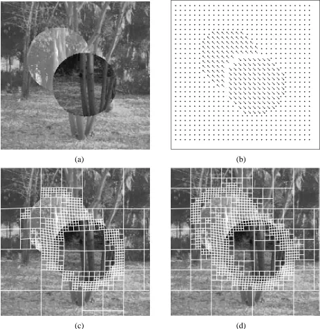
15 7 Quadtree spline motion estimation (Two Discs (SRI Trees) sequence): (a) input

image, (b) true flow, (c) split technique, (d) merge technique.

: : : : : : : : : : :

17

8 Flow errorku;u k and residual normal flowku N i

kfor Two Discs (SRI Trees)

sequence. Note how most of the errors are concentrated near the motion

disconti-nuities and especially the disoccluded region in the center.

: : : : : : : : : : : :

21

9 Hamburg Taxi sequence: estimated quadtree and estimated flow, merging

s

= 8

patches in a 3-level pyramid.

: : : : : : : : : : : : : : : : : : : : : : : : : : : :

21

10 Flower Garden sequence: estimated quadtree and estimated flow, merging

s

=4

: : : : : : : : : : : : : : : : : : : : : : : : : : : :

22

11 Michael Otte’s sequence: estimated quadtree and estimated flow, merging

s

= 8

: : : : : : : : : : : : : : : : : : : : : : : : : : : :

23

List of Tables

(7)

1 Introduction 1

1 Introduction

One of the fundamental tradeoffs in designing motion estimation and stereo matching algorithms is selecting the size of the windows or filters to be used in comparing portions of corresponding

im-ages. Using larger windows leads to better noise immunity through averaging and can also

disam-biguate potential matches in areas of weak texture or potential aperture problems. However, larger windows fail where they straddle motion or depth discontinuities, or in general where the motion

or disparity varies significantly within the window.

Many techniques have been devised to deal with this problem, e.g., using adaptively-sized win-dows in stereo matching. In this paper, we present a technique for recursively subdividing an image

into square patches of varying size and then matching these patches to subsequent frames in a way

which preserves inter-patch motion continuity. Our technique is an extension of the spline-based

image registration technique presented in [Szeliski and Coughlan, 1994], and thus has the same

advantages when compared to correlation-based approaches, i.e., lower computational cost and the

ability to handle large image deformations.

As a first step, we show how using hierarchical basis splines instead of regular splines can lead to faster convergence and qualitatively perform a smoothing function similar to

regulariza-tion. Then, we show how selectively setting certain nodes in the hierarchical basis to zero leads

to an adaptive hierarchical basis. We can use this idea to build a spline defined over a quadtree domain, i.e., a quadtree spline. To determine the size of the patches in our adaptive basis, i.e., the

shape of the quadtree, we develop both split and merge techniques based on the residual errors in the current optical flow estimates.

While this paper deals primarily with motion estimation (also known as image registration or

optical flow computation), the techniques developed here can equally well be applied to stereo

match-ing. In our framework, we view stereo as a special case of motion estimation where the epipolar

geometry (corresponding lines) are known, thus reducing a two-dimensional search space at each

pixel to a one-dimensional space. Our techniques can also be used as part of a direct method which

simultaneously solves for projective depth and camera motion [Szeliski and Coughlan, 1994]. The adaptive hierarchical basis splines developed in this paper are equivalent to adaptively

sub-dividing global parametric motion regions while maintaining continuity between adjacent patches.

We can therefore implement a continuum of motion models ranging from a single global (e.g.,

(8)

2 2 Previous work

algorithm as a parallel feature tracker for very long motion sequences where image deformations

may be significant [Szeliski et al., 1995].

The motion estimation algorithms developed in this paper can be used in a number of applica-tions. Examples include motion compensation for video compression, the extraction of 3D scene

geometry and camera motion, robot navigation, and the registration of multiple images, e.g., for

medical applications. Feature tracking algorithms based on our techniques can be used in human interface applications such as gaze tracking or expression detection, in addition to classical robotics

applications.

The remainder of the paper is structured as follows. Section 2 presents a review of relevant pvious work. Section 3 gives the general problem formulations for image registration. Section 4

re-views the spline-based motion estimation algorithm. Section 5 shows how hierarchical basis func-tions can be used to accelerate and regularize spline-based flow estimation. Section 6 presents our

novel quadtree splines and discusses how their shape can be estimated using both split and merge

techniques. Section 7 discusses the relationship of adaptive hierarchical basis splines to multiscale Markov Random Fields. Section 8 presents experimental results based on some commonly used

motion test sequences. We close with a comparison of our approach to previous algorithms and a

discussion of future work.

2 Previous work

Motion estimation has long been one of the most actively studied areas of computer vision and image processing [Aggarwal and Nandhakumar, 1988; Brown, 1992]. Motion estimation

algo-rithms include optical flow (general motion) estimators, global parametric motion estimators,

con-strained motion estimators (direct methods), stereo and multiframe stereo, hierarchical (coarse-to-fine) methods, feature trackers, and feature-based registration techniques. We will use this rough

taxonomy to briefly review previous work, while recognizing that these algorithms overlap and that

many algorithms use ideas from several of these categories.

The general motion estimation problem is often called optical flow recovery [Horn and Schunck,

1981]. This involves estimating an independent displacement vector for each pixel in an image.

Approaches to this problem include gradient-based approaches based on the brightness constraint

(9)

2 Previous work 3

and Bergen, 1985; Heeger, 1987; Fleet and Jepson, 1990; Weber and Malik, 1993], and

regulariza-tion [Horn and Schunck, 1981; Hildreth, 1986; Poggio et al., 1985]. Nagel [1987], Anandan [1989], and Otte and Nagel [1994] provide comparisons and derive relations between different techniques,

while Barron et al. [1994] provide some numerical comparisons.

Global motion estimators [Lucas, 1984; Bergen et al., 1992] use a simple flow field model

pa-rameterized by a small number of unknown variables. Examples of global motion models include

affine and quadratic flow fields. In the taxonomy of Bergen et al. [1992], these fields are called parametric motion models, since they can be used locally as well (e.g., affine flow can be estimated

at every pixel). The spline-based flow fields we describe in the next section can be viewed as local

parametric models, since the flow within each spline patch is defined by a small number of control

vertices.

Global methods are most useful when the scene has a particularly simple form, e.g., when the

scene is planar. These methods can be extended to more complex scenes, however, by using a col-lection of global motion models. For example, each pixel can be associated with one of several

global motion hypotheses, resulting in a layered motion model [Wang and Adelson, 1993; Jepson

and Black, 1993; Etoh and Shirai, 1993; Bober and Kittler, 1993]. Alternatively, a single image can

be recursively subdivided into smaller parametric motion patches based on estimates of the current

residual error in the flow estimate [M¨uller et al., 1994]. Our approach is similar to this latter work,

except that it preserves inter-patch motion continuity, and uses both split and merge techniques.

Stereo matching [Barnard and Fischler, 1982; Quam, 1984; Dhond and Aggarwal, 1989] is

traditionally considered as a separate sub-discipline within computer vision (and, of course, pho-togrammetry), but there are strong connections between it and motion estimation. Stereo can be

viewed as a simplified version of constrained motion estimation where the epipolar geometry is

given, so that each flow vector is constrained to lie along a known line. While stereo is traditionally

performed on pairs of images, more recent algorithms use sequences of images (multiframe stereo or motion stereo) [Bolles et al., 1987; Matthies et al., 1989; Okutomi and Kanade, 1993]. The idea

of using adaptive window sizes in stereo [Okutomi and Kanade, 1992; Okutomi and Kanade, 1994]

is similar in spirit to the idea used in this paper, although their algorithm has a much higher com-putational complexity.

Hierarchical (coarse-to-fine) matching algorithms have a long history of use both in stereo

(10)

4 3 General problem formulation

smaller, lower-resolution images and then use these to initialize higher-resolution estimates. Their

advantages include both increased computation efficiency and the ability to find better solutions by escaping from local minima.

The algorithm presented in this paper is also related to patch-based feature trackers [Lucas and

Kanade, 1981; Rehg and Witkin, 1991; Tomasi and Kanade, 1992]. It differs from these previous approaches in that we use patches of varying size, we completely tile the image with patches, and

we have no motion discontinuities across patch boundaries. Our motion estimator can be used as

a parallel, adaptive feature tracker by selecting spline control vertices with low uncertainty in both motion components [Szeliski et al., 1995].

3 General problem formulation

The general motion estimation problem can be formulated as follows. We are given a sequence of

images

I

t

(

xy

)which we assume were formed by locally displacing a reference image

I

(

xy

)with

horizontal and vertical displacement fields1

u

t

(

xy

)and

v

t

(

xy

), i.e.,

I

t (

x

+

u

t

y

+

v

t

)=

I

(

xy

)

:

(1)

Each individual image is assumed to be corrupted with uniform white Gaussian noise. We also

ignore possible occlusions (“foldovers”) in the warped images.

Given such a sequence of images, we wish to simultaneously recover the displacement fields

(

u

t

v

t

)and the reference image

I

(

xy

). The maximum likelihood solution to this problem is well

known and consists of minimizing the squared error

X

t Z Z

I

t (

x

+

u

t

y

+

v

t

);

I

(

xy

)]

2

dxdy:

(2)

In practice, we are usually given a set of discretely sampled images, so we replace the above inte-grals with summations over the set of pixelsf(

x

i

y

i )g.

If the displacement fields

u

tand

v

tat different times are independent of each other and the

refer-ence intensity image

I

(

xy

)is assumed to be known, the above minimization problem decomposes

into a set of independent minimizations, one for each frame. For now, we will assume that this is

i )]

2

:

(3)

1

(11)

3 General problem formulation 5

I

y

v

i

] 2

where

I

=

I

1

;

I

0 and

r

I

1

=(

I

x

I

y

)is the intensity gradient.

i )+

b

]

2

where

b

and

c

are the (per-frame) brightness and contrast correction terms. Both of these parameters can be estimated concurrently with the flow field at little additional cost. Their inclusion is most

useful in situations where the photometry can change between successive views (e.g., when the

images are not acquired concurrently).

Another way to generalize the criterion is to replace the squaring function with a non-quadratic

penalty function, which results in a robust motion estimator which can reject outlier measurements [Black and Anandan, 1993; Bober and Kittler, 1993; Black and Rangarajan, 1994]. Another

possi-bility is to weight each squared error term with a factor proportional to

1

2 I +

2 u

jr

I

j 2

where

2 I

and

2 u

are the variances of the image and derivative noise, which can compensate for noise

in the image derivative computation [Simoncelli et al., 1991]. To further increase noise immunity,

the intensity images used in (3) can be replaced by filtered images [Burt and Adelson, 1983]. The above minimization problem typically has many local minima. Several techniques are

com-monly used to find a more globally optimal estimate. For example, the SSD algorithm performs the

summation at each pixel over an

m

window (typically55) [Anandan, 1989]. More recent

i

v

i

[image:12.612.196.414.100.264.2]

)

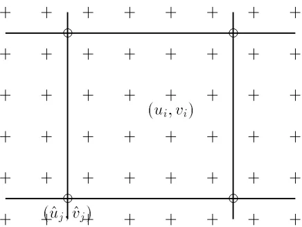
Figure 1: Displacement spline: the spline control verticesf(^

u

j

^

v

j

)gare shown as circles () and

al., 1992; Szeliski and Coughlan, 1994]. One can observe, however, that motion estimates at

indi-vidual pixels are never truly independent. Both local correlation windows (as in SSD) and global

smoothness constraints aggregate information from neighboring pixels. The resulting displacement

estimates are therefore highly correlated. While it is possible to analyze the correlations induced by overlapping windows [Matthies et al., 1989] and regularization [Szeliski, 1989], the procedures

are cumbersome and rarely used. For these reasons, we have chosen in our work to represent the motion field as a spline, which is a representation which falls in between per-pixel motion estimates

and purely global motion estimates.

4 Spline-based flow estimation

Our approach is to represent the displacements fields

u

(

xy

)and

v

(

xy

)as two-dimensional splines

controlled by a smaller number of displacement estimates

u

^ j and

^

v

j which lie on a coarser spline

u

i

= X

^

(13)

4.1 Function minimization 7

where the

B

i.e.,

B

j

(

xy

) =

B

(

x

;

x

^ j

y

;

y

^ j

). We have studied five different interpolation functions: (1)

block, (2) linear on squares, (3) linear on triangles, (4) bilinear, and (5) biquadratic [Szeliski and

Coughlan, 1994]. In practice, we most often use the bilinear bases. We also impose the condition

that the spline control grid is a regular subsampling of the pixel grid,

x

^ j =

mx

i, ^

y

j =

my

i, so that

each set of

m

pixels corresponds to a single spline patch.

4.1 Function minimization

To recover the local spline-based flow parameters, we need to minimize the cost function (3) with

respect to thef^

u

j

^

v

j

g. We do this using a variant of the Levenberg-Marquardt iterative non-linear

minimization technique [Press et al., 1992]. First, we compute the gradient of

E

in (3) with respect to each of the parameters

u

^

j and ^

v

j,

g

u j

@E

@

u

^

j =2

X

i

e

i

G

x i

w

ij

g

v j

@E

@

v

^

j =2

X

,

(

G

x i

G

y i

)=r

I

1

(

x

i

+

u

i

y

i

+

v

i

) (7)

(14)

8 4 Spline-based flow estimation

For the Levenberg-Marquardt algorithm, we also require the approximate Hessian matrix A

where the second-derivative terms are left out. The matrixAcontains entries of the form

ij

w

ik (

G

x i ) 2

a

uv jk =

a

v u jk = 2 X i

@e

i

@

u

^ j

@e

i

@

^

v

k

=2 X

i

w

ij

w

ik

G

x i

G

y

i (8)

a

v v jk

= 2 X

i

@e

i

@

v

^ j

@e

i

@

v

^ k

=2 X

i

w

ij

w

ik (

G

y i )

2

:

The entries ofAcan be computed at the same time as the energy gradients.

The Levenberg-Marquardt algorithm proceeds by computing an increment uto the current

displacement estimateuwhich satisfies

(A+

I)u =;g

(9)

whereuis the vector of concatenated displacement estimates f^

u

j

^

v

j

g,gis the vector of

concate-nated energy gradientsf

g

u j

g

v j

g, and

is a stabilization factor which varies over time [Press et al.,

1992]. To solve this large, sparse system of linear equations, we use preconditioned gradient de-scent

u=;

B ;1

g=;

g~ (10)

whereB= ^

A+

I, and ^

A =block diag(A)is the set of22block diagonal matrices defined in

(9) with

j

=

k

, andg~ =B ;1

gis called the preconditioned residual vector. 3

An optimal value for

can be computed at each iteration by minimizing

E

(

d)

2

d T

Ad;2

d T

g

i.e., by setting

=(dg )

=

(d T

Ad), whered= ~

gis the direction vector for the current step. See

[Szeliski and Coughlan, 1994] for more details on our algorithm implementation.

To handle larger displacements, we run our algorithm in a coarse-to-fine (hierarchical)

fash-ion. A Gaussian image pyramid is first computed using an iterated 3-point filter [Burt and Adelson, 1983]. We then run the algorithm on one of the smaller pyramid levels, and use the resulting flow

estimates to initialize the next finer level (using bilinear interpolation and doubling the displacement

magnitudes).

3

(15)

4.1 Function minimization 9

(a) (b)

(c) (d)

Figure 2: Example of general flow computation: (a) input image, (b)–(d) flow estimates for

m

=64,

(16)

10 5 Hierarchical basis splines

Figure 2 shows an example of the flow estimates produced by our technique. The input image

techniques have been developed to overcome this problem. Coarse-to-fine techniques [Quam, 1984; Anandan, 1989] can help, but often don’t converge as quickly to the optimal solution as

multi-grid techniques [Terzopoulos, 1986]. Conjugate gradient descent can also be used, especially for

non-linear problems such as shape-from-shading [Simchony et al., 1989]. Perhaps the most ef-fective technique is a combination of conjugate gradient descent with hierarchical basis functions

[Yserentant, 1986], which has been applied both to interpolation problems in stereo matching [Szeliski,

1990] and to shape-from-shading [Szeliski, 1991].

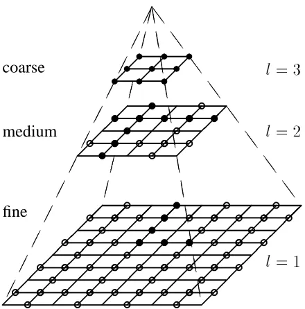
Hierarchical basis functions are based on using a pyramidal representation for the data [Burt and

Adelson, 1983], where the number of nodes in the pyramid is equal to the original number of nodes at the finest level (Figure 3). To convert from the hierarchical basis representation to the usual

fine-level representation (which is called the nodal basis representation [Yserentant, 1986]), we start at

the coarsest (smallest) level of the pyramid and interpolate the values at this level, thus doubling the resolution. These interpolated values are then added to the hierarchical representation values

at the next lower level, and the process is repeated until the nodal representation is obtained.4

This

process can be written algorithmically as

procedure

S

for

l

=

L

;1down to1

4

(17)

5 Hierarchical basis splines 11 ; ; ; ; ; ; ; ; ; ; ; ; ; ; ; ; ; ; ; ; ; ; ; ; ; ; ; ; ; ; ; ; ; ; ; ; ; ; ; ; ; ; ; ; ; ; ; ; ; ; ; ; ; ; ; ; ; ; ; ; ; ; ; ; ; ; ; ; ; ; ; ; ; ; ; ; ; ; ; ; ; ; ; ; ; ; ; ; ; ; ; ; ; ; ; ; ; ; E E E E E E E E E E E E E E E E E E E E E E E E S S S S S S S S S S S S S S S S fine medium coarse

l

=1

l

=2

l

=3

c c c c c c c c c c c c c c c c c c c c c c c c c c c c c c c c c c c c

c c c c c c c c c c c c c c c c c c

s s

s s s c c c c c c c c c c

c c c c c c c c c c

s s

s

[image:17.612.195.415.104.327.2]

s s s s s s s s s s s s s s

Figure 3: Multiresolution pyramid

The multiple resolution levels are a schematic representation of the hierarchical basis spline. The

circles indicate the nodes in the hierarchical basis. Filled circles () are free variables in the quadtree

spline (Section 6), while open circles () must be zero (see Figure 6).

for

j

2M l u

l j

=u^ l j + P k 2Nj ~

w

jk ^ u l+1 k

end

S

.

In this procedure, each node is assigned to one of the level collectionsM

l (the circles in Figure

3). Each node also has a number of “parent nodes”N

j on the next coarser level that contribute to

its value during the interpolation process. The

w

~

jk are the weighting functions that depend on the

particular choice of interpolation function. For the examples shown in this paper, we use bilinear interpolation, since previous experiments suggest that this is a reasonable choice for the interpolator

[Szeliski, 1990].

We can write the above process algebraically as

u =Su~ =S 1 S 2

:::

S L;1 ~

(18)

12 5 Hierarchical basis splines with (S l ) jk = 8 > > > < > > > :

1 if

j

=

k

~

w

jk if

j

2M

land

k

2N

j 0 otherwise

and~

uis the hierarchical basis representation. Using a hierarchical basis representation for the flow

field is equivalent to usingSS T

as a preconditioner, i.e.,~g = SS T

g[Axelsson and Barker, 1984;

Szeliski, 1990]. The transformationSS T

can be used as a preconditioner because the influence of

hierarchical bases at coarser levels (which are obtained from theS T

operation) are propagated to the nodal basis at the fine level through theSoperation. To evaluateS

T

, i.e., to convert from the

nodal basis representation to the hierarchical basis representation, we use the procedure

procedure

S

T

for

l

=1to

L

;1

for

k

2M l+1 ^ u l+1 k =u l+1 k + P j:k 2N j ~

w

jk ^ u l j

end

S

T

.

When combining hierarchical basis preconditioning with the block diagonal preconditioning in (10), we have several choices. We can apply the block diagonal preconditioning first,g~=SS

T B

;1 g,

or second,~g = B ;1

SS T

g, or we can interleave the two preconditionersg~ = SB ;1

S T

g, org~ = ^ B ;T SS T ^

Bg, where ^ B =B

1

2. The latter two operations correspond to well-defined

precondition-ers (i.e., optimization under a change of basis), while the first two are easier to implement. In our

current work, we use the first form, i.e., we apply block preconditioning first, and then use sweep up and then down the hierarchical basis pyramid to smooth the residual. In future work, we plan to

develop optimal combinations of block diagonal and hierarchical basis preconditioning.

To summarize our algorithm (Figure 4), we keep both the hierarchical and nodal representations, and map between the two as required. For accumulating the distances and gradients required in

(9), we compute the image flows and the derivatives with respect to the parameters in the nodal

basis. We then use the hierarchical basis to smooth the residual vector gbefore selecting a new

conjugate direction and computing the optimal step size. Using this technique not only makes the

convergence faster but also propagates local corrections over the whole domain, which tends to

smooth the resulting flow significantly.

(19)

5 Hierarchical basis splines 13

0

:

0

= 0

d ;1

=0 1

:

g

n

= ;r

E

(u) 2

:

y g~

n = SZS T B ;1 g n 3

:

n

y S =mapping from hierarchical to nodal basis, B =blo ckdiag(A)

[image:19.612.164.447.125.331.2]

Z =0/1 matrix for quadtree spline basis (Section 6).

Figure 4: Hierarchical basis preconditioned conjugate gradient algorithm

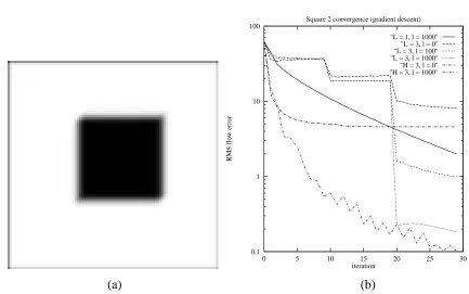
0.1 1 10 100

0 5 10 15 20 25 30

RMS flow error

iteration

Square 2 convergence (gradient descent)

"L = 1, l = 1000" "L = 3, l = 0" "L = 3, l = 100" "L = 3, l = 1000" "H = 3, l = 0" "H = 3, l = 1000"

(a) (b)

(a) input image, (b) convergence plot (error vs. iteration number)

[image:19.612.83.516.365.636.2]

(20)

14 6 Quadtree (adaptive resolution) splines

Figure 5a shows one image in the sequence, while Figure 5b shows the convergence rates for regular

gradient descent (

L

=1), coarse-to-fine estimation (

L

=3), and preconditioning with hierarchical

basis functions (

H

=3), with different amounts of regularization (

1

= 0

100

1000). As we can

see from these results, adding more regularization results in a more accurate solution (this is because

the true flow is a single constant value), using coarse to fine is quicker than single-level relaxation, and hierarchical basis preconditioning is faster than coarse-to-fine relaxation. It is interesting to

note that using hierarchical basis functions even without regularization quickly smooths out the

solution and outperforms coarse-to-fine without regularization.

6 Quadtree (adaptive resolution) splines

While hierarchical basis splines can help accelerate an estimation algorithm or even to add extra smoothness to the solution, they do not in themselves solve the problem of having adaptively-sized

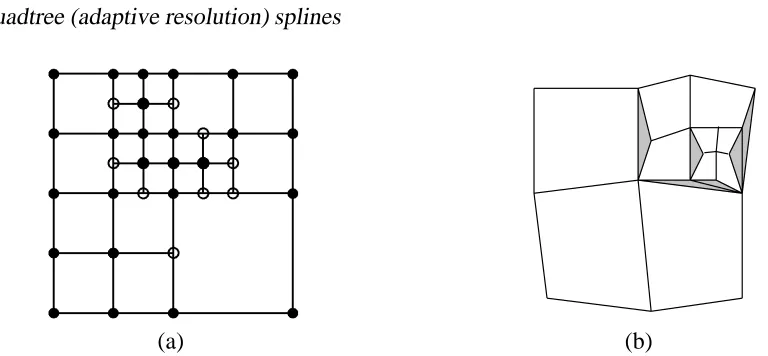
patches. For this, we will use the idea of quadtree splines, i.e., splines defined on a quadtree domain. A quadtree is a 2-D representation built by recursively subdividing rectangles into four pieces

(Fig-ure 6) [Samet, 1989]. The basic concept of a quadtree spline is to define a continuous function over

a quadtree domain by interpolating numeric values at the corners of each spline leaf cell (square). However, because cells are non-uniformly subdivided, cracks or first-order discontinuities in the

in-terpolated function will arise (Figure 6b) unless a crack-filling strategy is used [Samet, 1989]. The

simplest strategy is to simply replace the values at the nodes along a crack edge (the white circles in Figure 6) with the average values of its two parent nodes along the edge. This is the strategy we

used in developing octree splines for the representation of multi-resolution distance maps in 3-D

pose estimation problems [Lavall´ee et al., 1991].

When the problem is one of iteratively estimating the values on the nodes in the quadtree spline, enforcing the crack-filling rule becomes more complicated. A useful strategy, which we developed

for estimating 3-D displacement fields in elastic medical image registration [Szeliski and Lavall´ee,

1994], is to use a hierarchical basis and to selectively zero out nodes in this basis. Observe that if in Figures 3 and 6a we set the values of the open circles () to zero in the hierarchical basis and then

re-compute the nodal basis usingS, the resulting spline has the desired continuity, i.e., nodes along

longer edges are the averages of their parents.

(21)

6 Quadtree (adaptive resolution) splines 15 t t t t t t t t t t t t t t d t t

t t d

t t t t t

d t t t t d d d t d dt dt dt d d dt d

[image:21.612.102.486.72.250.2]

(a) (b)

Figure 6: Quadtree associated with spline function, and potential cracks in quadtree spline (a) the nodes with filled circles () are free variables in the associated hierarchical basis, whereas

the open circles () (and also the nodes not drawn) must be zero (in the nodal basis, these nodes

are interpolated from their ancestors); (b) potential cracks in a simpler quadtree spline are shown

as shaded areas.

simply requiring a selective zeroing step between theS T

andSoperations (algebraically, we write

~

g=SZS T

g, whereZis a diagonal matrix with 1’s and 0’s on the diagonal—see Figure 4). 5

Second, it generalizes to splines of arbitrary order, e.g., we can build a

C

1

quadtree spline based on quadratic

B-splines using adaptive hierarchical basis functions. However, for higher-order splines, even more

nodes have to be zeroed in order to ensure that finer level splines do not affect nearby coarser (un-divided) cells. Third, as we will discuss in the next section, the adaptive hierarchical basis idea is

even more general than the quadtree spline, and corresponds to a specific kind of multi-resolution

prior model.

The quadtree spline as described here ensures that the function within any leaf cell (square

do-main) has a simple form (single polynomial description, no spurious ripples). An alternative way

of interpreting the quadtree in Figure 6a is that it specifies the minimum degree of complexity in each cell, i.e., that each square is guaranteed to have its full degrees of freedom (e.g., all 4 corners

have independent values in the bilinear case). In this latter interpretation, the open circles in the

hierarchical basis are not zeroed, and only the circles actually not drawn in Figure 6a are zeroed. In this approach, large squares can have arbitrarily-detailed ripples inside their domain resulting

5

Whenever theZmatrix changes, we also have to re-compute the quadtree spline usingu SZS ;1

u. TheS ;1

procedure is similar toS T

, but nowu^ j

^ u j

;w~ jk

(22)

16 6 Quadtree (adaptive resolution) splines

from fine-level basis functions near the square’s boundaries. To date, we have not investigated this

alternative possibility.

6.1 Subdivision strategy

The quadtree spline provides a convenient way to use adaptively-sized patches for motion

estima-tion, while maintaining inter-patch continuity. The question remains how to actually determine the

topology of the patches, i.e., which patches get subdivided and which ones remain large. Ideally, we would like each patch to cover a region of the image within which the parametric motion model

is valid. In a real-world situation, this may correspond to planar surface patches undergoing rigid motion with a small amount of perspective distortion (bilinear flow is then very close to projective

flow). However, usually we are not a priori given the required segmentation of the image. Instead,

we must deduce such a segmentation based on the adequacy of the flow model within each patch.

The fundamental tool we will use here is the concept of residual flow [Irani et al., 1992], recently used by M¨uller et al. [1994] to subdivide affine motion patches (which they call tiles). The residual

flow is the per-pixel estimate of flow required to register the two images in addition to the flow

currently being modeled by the parametric motion model. At a single pixel, only the normal flow can be estimated,

u N i

y i

)k+

(12)

where the intensity error

e

i and the gradient r

I

1

= (

G

x i

G

y i

)are given in (6–7). This measure

is different from that used in [Irani et al., 1992; M¨uller et al., 1994], who sum the numerator and denominator in (12) over a small neighborhood around each pixel.

To decide whether to split a spline patch into four smaller patches, we sum the magnitude of

the residual normal flowku N i

k over all the pixels in the patch and compare it to a threshold u.

6

Patches where the motion model is adequate should fall below this threshold, while patches which have multiple motions should be above. Starting with the whole image, we subdivide recursively

until either the p-norm residual falls below an acceptable value or the smallest patch size considered (typically 4-8 pixels wide) is reached.

Figures 7a–c show an example of a quadtree spline motion estimate produced with this

split-ting technique for a simple synthetic example in which two central disks are independently moving

6

Actually, we use ap;norm,( P

ku N i

k p

) 1=p

(23)

6.1 Subdivision strategy 17

(a) (b)

[image:23.612.74.537.136.611.2]

(c) (d)

Figure 7: Quadtree spline motion estimation (Two Discs (SRI Trees) sequence): (a) input image,

(24)

18 7 A Bayesian interpretation

against a textured background. The quadtree boundaries are warped to show the extent of the

esti-mated image motion (up and left for the top disc, down and right for the bottom disc). Note how the subdivision occurs mostly at the object boundaries, as would be expected. The most visible error

(near the upper right edge of the lower disc) occurs in an area of little image contrast and where the

motion is mostly parallel to the region contour.

An alternative to the iterative splitting strategy is to start with small patches and to then merge

adjacent patches with compatible motion estimates into larger patches (within the constraints of allowable quadtree topologies). To test if a larger patch has consistent flow, we compare the four

values along the edge of the patch and the value at the center with the average values interpolated

from the four corner cells (look at the lower left quadrant of Figure 6a to visualize this). The relative difference between the estimated and interpolated values,

d

= k^

u j

;u j

k q

k^u j

k 2

+ku j

k 2

<

d

where u

j is the interpolated value, must be below a threshold d (typically 0.25-0.5) for all five

nodes before the four constituent patches are allowed to be merged into a larger patch. Notice

that the quantityu^ j

;u

j is exactly the value of the hierarchical basis function at a node (at least

for bilinear splines), so we are in effect converting small hierarchical basis values close to be

ex-actly zero (this has a Bayesian interpretation, as we will discuss in the next section). Note also that this consistency criterion may fail in regions of little texture where the flow estimates are initially

unreliable, unless regularization is applied to make these flow fields more smooth.

Figure 7d shows an example of a quadtree spline motion estimate produced with this merging

technique. The results are qualitatively quite similar to the results obtained with the split technique.

7 A Bayesian interpretation

The connection between energy-based or regularized low-level vision problems and Bayesian esti-mation formulations is well known [Kimeldorf and Wahba, 1970; Marroquin et al., 1987; Szeliski,

1989]. In a nutshell, it can be shown that the energy or cost function being minimized can be

con-verted into a probability distribution over the unknowns using a Gibbs or Boltzmann distribution,

(25)

7 A Bayesian interpretation 19

(typically the squared error terms between the measurements and their predicted values) and a prior

model (which usually corresponds to the stabilizer or smoothing term), i.e.,

E(u)=E d

(u

d)+E p

(u) ,

p

(u)/

(u

d)

p

(u) (13)

It then becomes straightforward to make use of robust statistical models by simply modifying the

appropriate energy terms [Black and Anandan, 1993; Black and Rangarajan, 1994].

The basic spline-based flow model introduced in [Szeliski and Coughlan, 1994] is already a valid prior model, since it restricts the family of functions to the smooth set of tensor-product splines.

In most cases, a small amount of intensity variation inside each spline patch is sufficient to ensure

that a unique, well-behaved solution exists. However, just to be on the safe side, it is easy to add a small amount of regularization with quadratic penalty terms on theu^

j’s and their finite differences.

Hierarchical basis splines, as well as other multilevel representations such as overcomplete

pyra-mids can be viewed as multiresolution priors [Szeliski and Terzopoulos, 1989]. There are two ba-sic approaches to specifying such a prior. The first, which we use in our current work, is to simply

view the hierarchical basis as a preconditioner, and to define the prior model over the usual nodal basis [Szeliski, 1990]. The alternative is to define the prior model directly on the hierarchical

ba-sis, usually assuming that each basis element is statistically independent from the others (i.e., that

the covariance matrix is diagonal) [Szeliski and Terzopoulos, 1989; Pentland, 1994]. An extreme example of this is the scale-recursive multiscale Markov Random Fields introduced in [Chin et al.,

1993], whose special structure makes it possible to recover the field in a single sweep through the

pyramid. Unfortunately, their technique is based on a piecewise-constant model of flow, which re-sults in recovered fields that have excessive “blockiness” [Luettgen et al., 1994].

Within this framework, adaptive hierarchical basis splines can be viewed as having a more

com-plex multiresolution prior where each hierarchical node has a non-zero prior probability of being exactly zero. The split and merge algorithms can be viewed as simple heuristic techniques designed

to recover the underlying motion field and to decide which nodes are actually zero. More

sophisti-cated techniques to solve this problem would include simulated annealing [Marroquin et al., 1987]

and mean-field annealing [Geiger and Girosi, 1991].

41

18

:

11

[image:26.612.110.497.108.232.2]

100%

Table 1: Summary of Two Discs (SRI Trees) results

8 Experimental results

To investigate the performance of our quadtree spline-based motion estimator, we use the

synthet-ically generated Two Discs (SRI Trees) sequence shown in Figure 7, for which we know the true motion (Figure 7b). The results of our spline-based motion estimator for various choices of

win-dow size

s

, as well as the results with both the split and merge techniques, are shown in Table 1. The experiments show that the optimal fixed window size is

s

=8, and that both split and merge

techniques provide slightly better results. The relatively small difference is error between the

vari-ous techniques is due to most of the error being concentrated in the regions where occlusions occur (Figure 8). Adding an occlusion detection process to our algorithm should help reduce the errors

in these regions.

We also tested our algorithm on some of the standard motion sequences used in other recent motion estimation papers [Barron et al., 1994; Wang and Adelson, 1993; Otte and Nagel, 1994].

The results on the Hamburg Taxi sequence are shown in Figure 9, where the independent motion

of the three moving cars can be clearly distinguished. Notice that the algorithm was also able to pick out the small region of the moving pedestrian near the upper left corner.

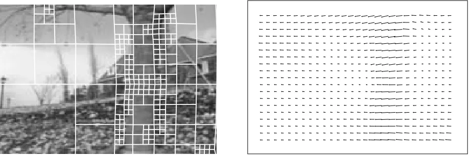
The result on the Flower Garden sequence are shown in Figure 10. Here, the trunk of the tree

is clearly segmented from the rest of the scene. The top of the flower garden, on the other hand, is not clearly segmented from the house and sky, since it appears that the

C

0

continuous motion field

represented by the splines is an adequate description.7

The final sequence which we studied is the table of marble blocks acquired by Michael Otte

7

(27)

[image:27.612.97.536.129.340.2]

= 8

estimate by first computing motion estimates with fewer frames (this is because gradient descent

gets trapped in local minima when the inter-frame displacements become large).

When the motion is not linear, i.e., we have a non-zero acceleration, we cannot perform a single batch optimization. Instead, we can compute a separate flow field between each pair of images,

using the previous flow as an initial guess. Alternatively, we can compute the motion between a base

image and each successive image, using a linear predictoru t

= u t;1

+(u t;1

;u t;2

). This latter

approach is useful if we are trying to track feature points without the problem of drift (accumulated

error) which can occur if we just use inter-frame flows.

The linearly predicted multiframe motion estimator forms the basis of our parallel extended

im-age sequence feature tracker [Szeliski et al., 1995]. To separate locations in the imim-age where

fea-tures are being tracked reliably from uninformative or confusing regions, we use a combination of the local Hessian estimate (9) and the local intensity error within each spline patch. This is similar

to Shi and Tomasi’s tracker [Shi and Tomasi, 1994], except that we use bilinear patches stitched

together by the spline motion model, which yields better stability than isolated affine patches.

(30)

24 10 Discussion and Conclusions

after inter-level transfers in the coarse to fine algorithm, or after splitting in the quadtree spline

es-timator, we search around the current(

uv

)estimate by trying a discrete set of nearby(

uv

)values

(as in SSD algorithms [Anandan, 1989]). However, because we must maintain spline continuity,

we cannot make the selection of best motion estimate for each patch independently. Instead, we

average the motion estimates of neighboring patches to determine the motion of each spline con-trol vertex.

In future work, we plan to extend our algorithm to handle occlusions in order to improve the

accuracy of the flow estimates. The first part, which is simpler to implement, is to simply detect

foldovers, i.e., when one region occludes another due to faster motion, and to disable error

con-tributions from the occluded background. The second part would be to add an explicit occlusion

model, which is not as straightforward because our splines are currently

C

0

continuous. In other

work, we would also like to study the suitability of our method as a robust way to bootstrap layered motion models. We also plan to test our technique on standard stereo problems.

10 Discussion and Conclusions

The quadtree-spline motion algorithm we have developed provides a novel way of computing an ac-curate motion estimate while performing an initial segmentation of the motion field. Our approach

optimizes the same stability versus detail tradeoff as adaptively-sized correlation windows, with-out incurring the large computational cost of overlapping windows and trial-and-error window size

adjustment. Compared to the recursively split affine patch tracker of [M¨uller et al., 1994], our

tech-nique provides a higher level of continuity in the motion field, which leads to more accurate motion estimates.

The general framework of quadtree splines and hierarchical basis functions is equally applicable

to other computer vision problems such as surface interpolation, as well as computer graphics and

numerical relaxation problems. It has already been applied successfully to the elastic registration of 3D medical images [Szeliski and Lavall´ee, 1994], and we plan to extend our approach to other

applications.

References

(31)

10 Discussion and Conclusions 25

the perception of motion. Journal of the Optical Society of America, A 2(2):284–299,

Febru-ary 1985.

[Aggarwal and Nandhakumar, 1988] J. K. Aggarwal and N. Nandhakumar. On the computation

of motion from sequences of images—a review. Proceedings of the IEEE, 76(8):917–935,

August 1988.

[Anandan, 1989] P. Anandan. A computational framework and an algorithm for the measurement of visual motion. International Journal of Computer Vision, 2(3):283–310, January 1989.

[Axelsson and Barker, 1984] O. Axelsson and V. A. Barker. Finite Element Solution of Boundary

Value Problems: Theory and Computation. Academic Press, Inc., Orlando, Florida, 1984.

[Barnard and Fischler, 1982] S. T. Barnard and M. A. Fischler. Computational stereo. Computing

Surveys, 14(4):553–572, December 1982.

[Barron et al., 1994] J. L. Barron, D. J. Fleet, and S. S. Beauchemin. Performance of optical flow

techniques. International Journal of Computer Vision, 12(1):43–77, January 1994.

[Bergen et al., 1992] J. R. Bergen, P. Anandan, K. J. Hanna, and R. Hingorani. Hierarchi-cal model-based motion estimation. In Second European Conference on Computer Vision

(ECCV’92), pages 237–252, Springer-Verlag, Santa Margherita Liguere, Italy, May 1992.

[Black and Anandan, 1993] M. J. Black and P. Anandan. A framework for the robust estimation of

optic flow. In Fourth International Conference on Computer Vision (ICCV’93), pages 231– 236, IEEE Computer Society Press, Berlin, Germany, May 1993.

[Black and Rangarajan, 1994] M. J. Black and A. Rangarajan. The outlier process: Unifying line

processes and robust statistics. In IEEE Computer Society Conference on Computer Vision

and Pattern Recognition (CVPR’94), pages 15–22, IEEE Computer Society, Seattle,

Wash-ington, June 1994.

[Bober and Kittler, 1993] M. Bober and J. Kittler. Estimation of complex multimodal motion: An

approach based on robust statistics and hough transform. In British Machine Vision

Confer-ence, pages 239–248, BMVA Press, 1993.

[Bolles et al., 1987] R. C. Bolles, H. H. Baker, and D. H. Marimont. Epipolar-plane image

anal-ysis: An approach to determining structure from motion. International Journal of Computer

Vision, 1:7–55, 1987.

(32)

[Burt and Adelson, 1983] P. J. Burt and E. H. Adelson. The Laplacian pyramid as a compact image

code. IEEE Transactions on Communications, COM-31(4):532–540, April 1983.

[Chin et al., 1993] T. M. Chin, M. R. Luettgen, W. C. Karl, and A. S. Willsky. An estimation-theoretic perspective on image processing and the calculation of optic flow. In Advances in

Image Sequence Processing, Kluwer, March 1993.

[Dhond and Aggarwal, 1989] U. R. Dhond and J. K. Aggarwal. Structure from stereo—a re-view. IEEE Transactions on Systems, Man, and Cybernetics, 19(6):1489–1510,

Novem-ber/December 1989.

[Enkelmann, 1988] W. Enkelmann. Investigations of multigrid algorithms for estimation of optical

flow fields in image sequences. Computer Vision, Graphics, and Image Processing, :150–177,

1988.

[Etoh and Shirai, 1993] M. Etoh and Y. Shirai. Segmentation and 2D motion estimation by region

fragments. In Fourth International Conference on Computer Vision (ICCV’93), pages 192–

199, IEEE Computer Society Press, Berlin, Germany, May 1993.

[Fleet and Jepson, 1990] D. Fleet and A. Jepson. Computation of component image velocity from

local phase information. International Journal of Computer Vision, 5:77–104, 1990.

[Geiger and Girosi, 1991] D. Geiger and F. Girosi. Mean field theory for surface

reconstruc-tion. IEEE Transactions on Pattern Analysis and Machine Intelligence, PAMI-13(5):401–

412, May 1991.

[Heeger, 1987] D. J. Heeger. Optical flow from spatiotemporal filters. In First International

Con-ference on Computer Vision (ICCV’87), pages 181–190, IEEE Computer Society Press,

Lon-don, England, June 1987.

[Hildreth, 1986] E. C. Hildreth. Computing the velocity field along contours. In N. I. Badler

and J. K. Tsotsos, editors, Motion: Representation and Perception, pages 121–127, North-Holland, New York, New York, 1986.

[Horn and Schunck, 1981] B. K. P. Horn and B. G. Schunck. Determining optical flow. Artificial

Intelligence, 17:185–203, 1981.

[Irani et al., 1992] M. Irani, B. Rousso, and S. Peleg. Detecting and tracking multiple moving

objects using temporal integration. In Second European Conference on Computer Vision

(33)

[Jepson and Black, 1993] A. Jepson and M. J. Black. Mixture models for optical flow

computa-tion. In IEEE Computer Society Conference on Computer Vision and Pattern Recognition

(CVPR’93), pages 760–761, New York, New York, June 1993.

[Kimeldorf and Wahba, 1970] G. Kimeldorf and G. Wahba. A correspondence between Bayesian

estimation on stochastic processes and smoothing by splines. The Annals of Mathematical

Statistics, 41(2):495–502, 1970.

[Lavall´ee et al., 1991] S. Lavall´ee, R. Szeliski, and L. Brunie. Matching 3-d smooth surfaces with

their 2-d projections using 3-d distance maps. In SPIE Vol. 1570 Geometric Methods in

Com-puter Vision, pages 322–336, Society of Photo-Optical Instrumentation Engineers, San Diego,

July 1991.

[Lucas, 1984] B. D. Lucas. Generalized Image Matching by the Method of Differences. PhD

the-sis, Carnegie Mellon University, July 1984.

[Lucas and Kanade, 1981] B. D. Lucas and T. Kanade. An iterative image registration technique

with an application in stereo vision. In Seventh International Joint Conference on Artificial

Intelligence (IJCAI-81), pages 674–679, Vancouver, 1981.

[Luettgen et al., 1994] M. R. Luettgen, W. C. Karl, and A. S. Willsky. Efficient multiscale regu-larization with applications to the computation of optical flow. IEEE Transactions on Image

Processing, 3(1):41–64, January 1994.

[Mallat, 1989] S. G. Mallat. A theory for multiresolution signal decomposition: the wavelet

representation. IEEE Transactions on Pattern Analysis and Machine Intelligence,

PAMI-11(7):674–693, July 1989.

[Marroquin et al., 1987] J. Marroquin, S. Mitter, and T. Poggio. Probabilistic solution of ill-posed problems in computational vision. Journal of the American Statistical Association,

82(397):76–89, March 1987.

[Matthies et al., 1989] L. H. Matthies, R. Szeliski, and T. Kanade. Kalman filter-based algorithms for estimating depth from image sequences. International Journal of Computer Vision, 3:209–

236, 1989.

[M¨uller et al., 1994] J. R. M¨uller, P. Anandan, and J. R. Bergen. Adaptive-complexity registration

of images. In IEEE Computer Society Conference on Computer Vision and Pattern

(34)

[Nagel, 1987] H.-H. Nagel. On the estimation of optical flow: Relations between different

ap-proaches and some new results. Artificial Intelligence, 33:299–324, 1987.

[Okutomi and Kanade, 1992] M. Okutomi and T. Kanade. A locally adaptive window for signal

matching. International Journal of Computer Vision, 7(2):143–162, April 1992.

[Okutomi and Kanade, 1993] M. Okutomi and T. Kanade. A multiple baseline stereo. IEEE

Transactions on Pattern Analysis and Machine Intelligence, 15(4):353–363, April 1993.

[Okutomi and Kanade, 1994] M. Okutomi and T. Kanade. A stereo matching algorithm with an

adaptive window: Theory and experiment. IEEE Transactions on Pattern Analysis and

Ma-chine Intelligence, 16(9):920–932, September 1994.

[Otte and Nagel, 1994] M. Otte and H.-H. Nagel. Optical flow estimation: advances and compar-isons. In Third European Conference on Computer Vision (ECCV’94), pages 51–60,

Springer-Verlag, Stockholm, Sweden, May 1994.

[Pentland, 1994] A. P. Pentland. Interpolation using wavelet bases. IEEE Transactions on Pattern

Analysis and Machine Intelligence, 16(4):410–414, April 1994.

[Poggio et al., 1985] T. Poggio, V. Torre, and C. Koch. Computational vision and regularization

theory. Nature, 317(6035):314–319, 26 September 1985.

[Press et al., 1992] W. H. Press, B. P. Flannery, S. A. Teukolsky, and W. T. Vetterling.

Numeri-cal Recipes in C: The Art of Scientific Computing. Cambridge University Press, Cambridge,

England, second edition, 1992.

[Quam, 1984] L. H. Quam. Hierarchical warp stereo. In Image Understanding Workshop, pages 149–155, Science Applications International Corporation, New Orleans, Louisiana,

De-cember 1984.

[Rehg and Witkin, 1991] J. Rehg and A. Witkin. Visual tracking with deformation models. In

IEEE International Conference on Robotics and Automation, pages 844–850, IEEE Computer

Society Press, Sacramento, California, April 1991.

[Samet, 1989] H. Samet. The Design and Analysis of Spatial Data Structures. Addison-Wesley, Reading, Massachusetts, 1989.

[Shi and Tomasi, 1994] J. Shi and C. Tomasi. Good features to track. In IEEE Computer Society

Conference on Computer Vision and Pattern Recognition (CVPR’94), pages 593–600, IEEE

(35)

[Simchony et al., 1989] T. Simchony, R. Chellappa, and Z. Lichtenstein. Pyramid implementation

of optimal-step conjugate-search algorithms for some low-level vision problems. IEEE

Trans-actions on Systems, Man, and Cybernetics, SMC-19(6):1408–1425, November/December

1989.

[Simoncelli et al., 1991] E. P. Simoncelli, E. H. Adelson, and D. J. Heeger. Probability

distribu-tions of optic flow. In IEEE Computer Society Conference on Computer Vision and Pattern

Recognition (CVPR’91), pages 310–315, IEEE Computer Society Press, Maui, Hawaii, June

1991.

[Singh, 1990] A. Singh. An estimation-theoretic framework for image-flow computation. In Third

International Conference on Computer Vision (ICCV’90), pages 168–177, IEEE Computer

Society Press, Osaka, Japan, December 1990.

[Szeliski, 1989] R. Szeliski. Bayesian Modeling of Uncertainty in Low-Level Vision. Kluwer

Aca-demic Publishers, Boston, Massachusetts, 1989.

[Szeliski, 1990] R. Szeliski. Fast surface interpolation using hierarchical basis functions. IEEE

Transactions on Pattern Analysis and Machine Intelligence, 12(6):513–528, June 1990.

[Szeliski, 1991] R. Szeliski. Fast shape from shading. CVGIP: Image Understanding, 53(2):129–

153, March 1991.

[Szeliski and Coughlan, 1994] R. Szeliski and J. Coughlan. Hierarchical spline-based image

reg-istration. In IEEE Computer Society Conference on Computer Vision and Pattern Recognition

(CVPR’94), pages 194–201, IEEE Computer Society, Seattle, Washington, June 1994.

[Szeliski and Lavall´ee, 1994] R. Szeliski and S. Lavall´ee. Matching 3-D anatomical surfaces with non-rigid deformations using octree-splines. In IEEE Workshop on Biomedical Image

Anal-ysis, pages 144–153, IEEE Computer Society, Seattle, Washington, June 1994.

[Szeliski and Terzopoulos, 1989] R. Szeliski and D. Terzopoulos. Parallel multigrid algorithms

and computer vision applications. In Fourth Copper Mountain Conference on Multigrid

Methods, pages 383–398, Society for Industrial and Applied Mathematics, Copper Mountain,

Colorado, April 1989.

[Szeliski et al., 1995] R. Szeliski, S. B. Kang, and H.-Y. Shum. A Parallel Feature Tracker for

Ex-tended Image Sequences. Technical Report 95/2, Digital Equipment Corporation, Cambridge

Research Lab, April 1995.

(36)

Transactions on Pattern Analysis and Machine Intelligence, PAMI-8(2):129–139, March

1986.

[Tomasi and Kanade, 1992] C. Tomasi and T. Kanade. Shape and motion from image streams

under orthography: A factorization method. International Journal of Computer Vision,

9(2):137–154, November 1992.

[Wang and Adelson, 1993] J. Y. A. Wang and E. H. Adelson. Layered representation for motion

analysis. In IEEE Computer Society Conference on Computer Vision and Pattern Recognition

(CVPR’93), pages 361–366, New York, New York, June 1993.

[Weber and Malik, 1993] J. Weber and J. Malik. Robust computation of optical flow in a

multi-scale differential framework. In Fourth International Conference on Computer Vision

(ICCV’93), pages 12–20, IEEE Computer Society Press, Berlin, Germany, May 1993.

[Witkin et al., 1987] A. Witkin, D. Terzopoulos, and M. Kass. Signal matching through scale

space. International Journal of Computer Vision, 1:133–144, 1987.

[Yserentant, 1986] H. Yserentant. On the multi-level splitting of finite element spaces. Nu-merische Mathematik, 49:379–412, 1986.

Acknowledgements

We would like to thank John Wang and Michael Otte for providing us with the motion sequences