SRC Technical Note
1997 - 012
June 24, 1997
Online Throughput-Competitive Algorithm for
Multicast Routing and Admission Control
Ashish Goel, Monika Rauch Henzinger and Serge Plotkin
d i g i t a l
Systems Research Center130 Lytton Avenue Palo Alto, California 94301
http://www.research.digital.com/SRC/
Abstract
We present the first polylog-competitive online algorithm for the general multicast problem in the throughput model. The ratio of the number of re-quests accepted by the optimum offline algorithm to the expected number of requests accepted by our algorithm is O(logM(log n +log logM)log n),
whereMis the number of multicast groups and n is the number of nodes in
the graph. We show that this is close to optimum by presenting an(log n logM)
lower bound on this ratio for any randomized online algorithm against an oblivious adversary, whenMis much larger than the link capacities. We
also show that it is impossible to be competitive against an adaptive online adversary.
As in the previous online routing algorithms, our algorithm uses edge-costs when deciding on which is the best path to use. In contrast to the previ-ous competitive algorithms in the throughput model, our cost is not a direct function of the edge load. The new cost definition allows us to decouple the effects of routing and admission decisions of different multicast groups.
1
Introduction
Future high-speed communication networks such as ATM will use bandwidth-reservation in order to achieve Quality of Service (QoS) guarantees. Given a re-quest for a Virtual Circuit (VC), the router has to either accept or reject this rere-quest and, if it decides to accept it, allocate the requested bandwidth along a path con-necting the endpoints of the VC.
In case of multicast requests, the bandwidth has to be allocated along a tree spanning the nodes participating in the multicast group. In the general case, a multicast request specifies the user (endpoint) and the multicast group that this user wants to participate in. The router should either reject the request or accept it and allocate bandwidth along a path connecting the new endpoint with the already existing tree for this group.
In this paper we present the first polylog-competitive algorithm for the general multicast problem. Our algorithm is randomized since it is impossible to achieve polylog competitive ratio by a deterministic algorithm. The ratio of the number of requests accepted by the optimum offline algorithm to the expected number of requests accepted by our algorithm is O(logM(log n+log logM)log n), where
Mis the number of multicast groups and n is the number of nodes in the graph. If
each vertex is allowed to serve at most one multicast group, the competitive ratio simplifies to O(log3n).
studied. In particular, in [3] it was shown how to achieve O(log n)competitive ratio with respect to throughput for infinite duration requests, i.e. number of accepted requests, and O(log nT)ratio for requests that specify holding times (durations) upon arrival, where T is the longest duration. The randomized model where the durations are exponentially distributed and the arrivals are Poisson with unknown rates was considered in [9]. They describe a(1+)-competitive algorithm, where
depends on the ratio of the minimum capacity to maximum bandwidth of a single VC. Both [3] and [9] assume at least logarithmic ratio between maximum VC band-width and minimum link capacity. Similar results without this assumption were developed for special network topologies (see e.g. [10]). An optimal congestion-competitive online algorithm for multicast routing was presented in [1].
The techniques in the above mentioned papers can be used to solve several restricted multicast problems. In particular, [3] shows that if the participants in a single multicast group arrive together(“batch arrivals”), and the accept/reject deci-sion is for the whole multicast group, it is possible to achieve O(log n)competitive ratio. The case where we keep the restriction of batch arrivals, but allow rejection of some of the group members and acceptance of others is considered in [6].
Recently, Awerbuch and Singh has shown how to combine the “winner-picking” technique [2] with the techniques in [3] to achieve a polylog competitive ratio for the case where members of each multicast group arrive sequentially, i.e. the size and membership of the group is unknown upon its creation. Their algorithm can deal only with the non-interleaved case, i.e. when all the members of a particular multicast group arrive before a new group can be created.
It is not clear how to apply the algorithm and the analysis of [4] to the more general case, where the arrivals of requests belonging to different multicast groups are interleaved. The main problem is that their algorithm strongly depends on the fact that, at every instance, the algorithm is dealing with the construction of only a single multicast tree and all accept/reject decisions with respect to all existing multicast groups are already known.
As in [3], the algorithm in [4] uses edge costs the are exponential in the cur-rent link load. One of our contributions is a new definition of edge-costs that are independent of the specific accept/reject decisions made with respect to each mul-ticast group. This decoupling between mulmul-ticast groups is what allows us to apply the techniques in [3] and [2] to achieve a polylog competitive ratio for the general multicast problem.
A natural question to ask is if it is possible to make the competitive ratio inde-pendent ofM, the number of multicast group. We address this issue by showing
This is the first bound for this problem that is stronger than(log n).
The algorithm presented in this paper works against a semi-oblivious adver-sary, i.e. the adversary is allowed to look at the tree used by the online algorithm to service a multicast group only after all the requests for that group have been processed1. We show that no algorithm can do well against an adaptive online adversary.
As is customary for online algorithms, previous papers on multicast ignored the issue of computational complexity. In particular, the algorithm in [4] assumes an NP-hard computation at each routing decision. We show that it is possible to use the special properties of the Prize-Collecting Steiner tree algorithm in [8] to implement each step of our algorithm in polynomial time.
In Section 2 we introduce the model and the terminology. Section 3 describes the algorithm, and Section 5 presents the proof of the competitive ratio. Lower bounds are presented in Section 8. Appendix A explains how to implement each decision step of our online algorithm in polynomial time.
2
Model and Definitions
A request to join a multicast group specifies the group, the node that wants to join, and the amount of the requested bandwidth. The multicast routing and admission algorithm can either reject this “join” request or accept it and allocate the requested bandwidth along some path from the new node to the current tree associated with the requested multicast group. The algorithm is not allowed to allocate above link capacity.
We model the network as a capacitated graph with n nodes and m edges. For simplicity, we will assume that all edges have capacity u and all requests are for unit bandwidth. We also assume that the number of multicast groupsMis known
in advance. The issue of removing some of the assumptions is deferred to Sec-tion 7.
We also assume that u ≥ logµ, where µ is a parameter that is polynomial in n,Mdefined later.
2 We assume that multicast groups, once established, never
leave. The case where each multicast group has a “holding time” will be addressed in the full version of this paper.
1A semi-oblivious adversary is at least as powerful as an oblivious adversary.
3
The Algorithm
The online algorithm can be viewed as consisting of L = log n +logM
“vir-tual” algorithms for each one of theMmulticast groups. We call these algorithms
virtual because the routing and accept/reject decisions of these algorithms are not implemented. Instead, they only modify internal data structures and, in particu-lar the cost associated with each edge. The description of the cost computation is deferred to Section 4. For now, it is sufficient to assume that each edge has an as-sociated cost that is deterministic, depends only on the input sequence of requests, and is monotonically non-decreasing in time.
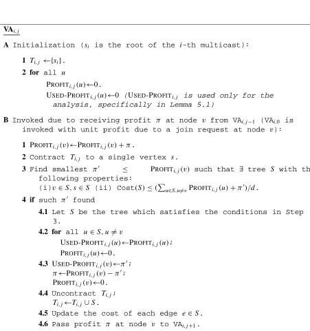
The j th virtual algorithm associated with the ith multicast – VAi,j – is shown
in Figure 1. The goal of VAi,j is to build a tree Ti,j. This tree spans some of the
nodes that requested to be added to the ith multicast group and that are already spanned by trees Ti,k, for k < i. In other words, a request is first generated at
VAi,1; if it immediately gets added to Ti,1, it is passed on to VAi,2, etc.
Each request to join the ith multicast group is considered as a potential unit of profit, and the virtual algorithms use (“consume”) this profit to “pay” for their trees. VAi,j can expand its tree Ti,j by adding a subtree only if it can pay for this
subtree. We will refer to these subtrees as “fragments”. As payment, VAi,j can use
only the profit that is on the nodes of this subtree and that was not used by VAi,k
for k < j (This is denoted by PROFITi,j(v)in Figure 1). More precisely, VAi,j
monitors the profit passed from VAi,j−1. Each time it getsπ units of profit at some
nodev, it addsπ to PROFITi,j(v). It then tries to find a fragment that includesv
such that the ratio of the unused profit associated with nodes of this fragment plus
π0is at least d =dT · 1
6L log n times the cost of adding this fragment to Ti,j, where
dT = 1/(mu) andπ0 ≤ PROFITi,j(v). The goal of the algorithm is to minimize
π0.
This subtree is added to the Ti,j, d times the cost of this tree is “consumed”,
and the rest of the profit (in fact, at most one unit) on the newly added nodes is bequeathed to Vi,j+1.
Observe that, since costs are increasing, the total profit used to construct Ti,j
is bounded by its final cost divided by d. Since VAi,j builds its tree in an online
VAi,j
A Initialization (si is the root of the i-th multicast):
1 Ti,j ←{si}.
2 for all u
PROFITi,j(u)←0.
USED-PROFITi,j(u)←0 (USED-PROFITi,j is used only for the
analysis, specifically in Lemma 5.1)
B Invoked due to receiving profit π at node v from VAi,j−1 (VAi,0 is
invoked with unit profit due to a join request at node v):
1 PROFITi,j(v)←PROFITi,j(v)+π.
2 Contract Ti,j to a single vertex s.
3 Find smallest π0 ≤ PROFITi,j(v) such that ∃ tree S with the
following properties:
(i)v ∈S,s∈ S (ii) Cost(S)≤(Pu∈S,u6=vPROFITi,j(u)+π0)/d.
4 if such π0 found
4.1 Let S be the tree which satisfies the conditions in Step
3.
4.2 for all u ∈S,u6=v
USED-PROFITi,j(u)←PROFITi,j(u);
PROFITi,j(u)←0.
4.3 USED-PROFITi,j(v)←π0;
π←PROFITi,j(v)−π0;
PROFITi,j(v)←0.
4.4 Uncontract Ti,j;
Ti,j←Ti,j ∪S.
4.5 Update the cost of each edge e∈ S.
[image:7.612.127.578.120.601.2]4.6 Pass profit π at node v to VAi,j+1.
Real(i)
1 Choose ηi ∈[1. . .L] such that Prob(ηi = j)=β·2j.
2 Follow the computation of VAi,ηi and whenever an edge gets added to
Ti,ηi, add that edge to the real tree being used to service the
i-th multicast group.
Figure 2: The Real algorithm for multicast group i.
vertices that contribute towards the profit collected by VAi,j−1.
The “real” algorithm is shown in Figure 2. For each multicast group, it ran-domly chooses one of the virtual algorithms and implements the construction of the tree built by this virtual algorithm. We set the probability of choosing VAi,j to
pj =β·2j, whereβ is chosen such that
PL
j=1pj =1.
Observe that if the i-th real algorithm has chosen VAi,j for a specific multicast,
it does not get the profit for the requests that were taken into account when VAi,j
was constructing its tree. Instead, it will get the profit for the later requests. In particular, it will get the profit that was inherited by VAi,j+1.
In Step 3 of the virtual algorithm (see Figure 1) we need to solve the maximal dense subtree problem, which is NP-hard. In Appendix A we show how a good-enough approximation can be obtained in polynomial time.
4
Edge Costs
In this section we define the cost metric and the way it is updated as a result of each new request. The cost metric is updated by the virtual algorithms and hence is deterministic.
The online algorithm constructs the cost metric as it goes along. When profit propagates from VAi,j−1 to VAi,j, we consider this an “event”. An event might
cause VAi,j to consume some profit and update its tree Ti,j. Let ce(k) denote
the cost of edge e after the k-th event. When the kth event occurs, the virtual algorithms use costs ce(k−1)for making their decision. These decisions are then
used to compute ce(k)in a deterministic fashion.
LetηE =(η1, . . . , ηM)represent the indices of the virtual algorithms chosen for
of choices. Define the load on an edge as 1/u times the number of trees it was used in by the real algorithm, and letλ(eη)E(k)represent the load on edge e after the
first k events have occurred, whereηErepresents the choices made by the Real al-gorithms. Since the random choices of the Real algorithms for different multicasts are independent, pηE =QM
i=1 pηi.
Let ce(0) = u for each edge e. Suppose costs c(0)to c(k−1)were already
computed. Then ce(k)is computed as follows.
ce(k)=u
X
E
η
pηEµλ(eη)E(k)
The value ofµ is set to 4m6log2M. The reason for this value will become
clear in Section 6. Observe that, givenηE, the expressionλ(eη)E(k) is deterministic,
and hence the costs ce(k)are deterministic as well.
Define X(ei,j)(k)as indicator variables, with Xie,j(k)being 1 if edge e is used by
VAi,j during the first k events and 0 otherwise. Notice that X(ei,j)(k)are
determin-istic quantities. Now,λ(eη)E(k) =(1/u)·
PM
i=1X
(i,ηi)
e (k). We can use this to rewrite
the cost ce(k):
ce(k)=u
X
E
η
M Y
i=1
pηi·µ
X(ei,ηi)(k)/u
Interchanging the order of the summation and the product, we get
ce(k)=u
M Y
i=1
L
X
j=1
pjµX
(i,j)
e (k)/u (1)
The above representation gives an easy way to compute ce(k)efficiently. Since
only one of the sums changes during any event, the online algorithm can recompute that sum and obtain the new costs.
The following claim follows from the way we construct the cost metric.
Claim 4.1 The cost ce(k)is the expectation of the quantity uµλe(k) whereλe(k)is
a random variable representing the load on edge e after k events.
5
Proof of competitiveness
groups with respect to the cost metric constructed by our algorithm. Here, by optimum trees we mean the trees constructed by the optimum offline algorithm.
Consider the ith multicast group, and let the number of requests satisfied by the optimal offline algorithm be r∗(i). Similarly, let r(i)be the profit obtained by the online algorithm. Letw∗(i)be the cost (in the final cost metric) of the tree Ti∗ used by the optimum algorithm to service multicast group i. We call a multicast group profitable if the optimal’s tree for this multicast group has a high profit to cost ratio in the final cost metric:
Definition 1 The i-th multicast group is profitable if wr∗∗((ii)) ≥dT, where dT = 1
mu.
We use the quantities R∗ and R to represent PM
i=1r∗(i) and
PM
i=1r(i),
re-spectively. Let P and U represent the set of profitable and unprofitable multicast groups, respectively. Also, we define R∗P =Pi∈Pr∗(i)and RU∗ =Pi∈Ur∗(i) = R∗−R∗P.
We first show (Lemma 5.2) that the online algorithm obtains almost as much profit from profitable groups as the optimal solution. Then we show that the total profit obtained by the online algorithm can only be poly-logarithmically smaller than optimal’s profit from unprofitable groups. To prove the latter claim, we take an indirect route. We use capacity constraints to argue that the quantity m RU∗ is bounded by the sum of the final costs of all edges (Lemma 5.3). Finally, we bound the final costs in terms of the expected profit obtained by the online algorithm (Lemma 5.7).
Consider the quantities PROFITi,j(v)and USED-PROFITi,j(v)at the end ie.
af-ter all requests have been received. Let Pi,j(v)=PROFITi,j(v)+USED-PROFITi,j(v).
The quantity Pi,j(v) denotes the profit consumed by VAi,j at node v. For any
set X of vertices, Pi,j(X) =
P
v∈X Pi,j(v). The definitions of PROFITi,j and
USED-PROFITi,j are similarly extended.
Lemma 5.1 Pi,j(Ti∗)≤3w∗(i)d log n.
Proof: O ur proof of this claim is different from the one presented in [4].
We first bound the quantity PROFITi,j(Ti∗). This contribution comes from
nodes in Ti∗ which do not belong to Ti,j. The profit consumed on these nodes
by VAi,j must be at mostw∗(i)d, else these nodes would have formed a fragment
on their own and been added to Ti,j.
Now we bound USED-PROFITi,j(Ti∗). This contribution comes from nodes
that belong to Ti,j. Recall that V Ai,j acquires Ti,j in tree fragments. Consider an
D such that all edges of the segment belong to the same fragment of Ti,j. Initially,
all segments are marked active. If two consecutive active segments on this tour belong to the same fragment, they are merged together along with the portion of the tour between between them to form a single segment. Let t(s)denote the event at which the edges of segment s were added to Ti,j.
Furthermore, we define a pr ed and succ relation on active segments such that pr ed(s,D)is the predecessor of s in tour D and succ(s,D)is the successor of s in D.
Let D0 = D. For h ≥ 1, let Hh = {s is an active segment of Dh−1,t(s) <
t(pr ed(s,Dh−1)),t(s) < t(succ(s,Dh−1))}. LetLh denote the remaining
seg-ments of Dh−1, and let Dh denote the tour Dh−1 with each segment inLh marked
inactive. The segments inHhremain active in Dh. As mentioned above,
consecu-tive acconsecu-tive segments are merged if they belong to the same fragment.
Note that for all h:
|Lh|>|Hh|.
This implies that there at most log n non empty setsLh. Let s ∈ Lh for some h.
Also, let s0be the successor or predecessor segment of s in Dh−1 with t(s0) <t(s)
and let p consists of the part of D between s and s0.
Assume USED-PROFITi,j(s)≥d(w∗(s)+w∗(p)). Letv ∈s be the node with
the last request in multicast i among all nodes in s. When the request atvarrived, the sum PROFITi,j(s)=Pu∈sPROFITi,j(u)is at least d(w∗(s)+w∗(p)), because PROFITi,j(s)is the source of USED-PROFITi,j(s). Thus, at that time we could have used at most d(w∗(s)+w∗(p))to add s+ p as a fragment. Since the algorithm always tries to create a fragment using the minimum amount of profit, we have:
USED-PROFITi,j(s)≤d(w∗(s)+w∗(p)). Considering that D visits every node twice it follows that
X
s∈Lh
USED-PROFITi,j(s)≤2w∗(i)d.
Summing over all values of h it follows that the profit consumed by V Ai,j from
all nodes which belong to T∗∩Ti,j is at most 2w∗(i)d log n. This completes the
proof of this lemma.
It is easy to see that, for profitable multicasts, the profit obtained by our online algorithm is high:
Proof: Since there are L levels, Lemma 5.1 guarantees that the total wasted profit for multicast group i is at most 3Lw∗(i)d log n. Plugging in d =dT ·6L log n1 and using the fact that i profitable implies that r∗(i)≥dTw∗(i), we obtain a bound of r∗(i)/2 on the wasted profit. Therefore, r(i) ≥r∗(i)/2 for all profitable groups i. Summing over all the profitable groups, we get the desired result.
Having bounded the profit from the profitable groups, we now concentrate on the unprofitable groups. Recall that ce is the cost of edge e at the end i.e. after all
the events have taken place, and that the costs are non-decreasing in time.
Lemma 5.3 m RU∗ ≤Pece
Proof: Let ke∗be the number of multicast groups which use edge e in the optimal offline solution. Consider the tree Ti∗used by the optimal to route the i-th multicast group. If this group is unprofitable then by definition r∗(i) ≤ mu1 Pe∈T∗
i ce. We sum this over all the unprofitable multicast groups, and then reverse the order of summation.
RU∗ ≤ 1 mu
X
i∈U
X
e∈Ti∗
ce
≤ 1 mu
X
e
ke∗ce
≤ 1 m
X
e
ce
The last inequality follows from the fact that the optimal offline is not allowed to exceed capacities, implying ke∗≤u.
Let wj(i) represent the cost incurred by VAi,j in constructing the tree Ti,j.
In other words, each tree fragment of Ti,j contributes towj(i) its cost associated
with the event of adding this fragment. We usew(i) to denotewη(i)(i), whereη
represents the chose of the real algorithm. Let rj(i)represent the profit consumed
in constructing this Ti,j. The following lemma implies that if the expected profit is
small, then the expected cost of the constructed trees is small as well.
Lemma 5.4 E(r(i)) ≥ (d/2)E(w(i)) − 1
M
, where w(i) is the cost paid by the Real algorithm for multicast group i.
Proof: If the real algorithm chooses to follow VAi,j, i.e.η(i)= j , then it will get
at least the profit used by VAi,j+1. Therefore:
E(r(i))≥
L−1
X
j=1
By definition, pj = pj+1/2, and hence
E(r(i))≥
L
X
j=2
pjrj(i)/2.
By construction:
E(w(i))=
L
X
j=1
pjwj(i)≤(1/d) L
X
j=1
pjrj(i).
Thus, we have
d·E(w(i))≤2E(r(i))+p1r1(i).
Now notice that r1(i) can be at most n, since each request brings in one unit of
profit, and there can be at most n requests for a single multicast group. Also, p1
PL
j=12j−1 = 1, which implies that p1/2 < 2−L. Substituting L = log n+
logM, we obtain E(r(i))≥(d/2)E(w(i))−
1
M
.
We remark that in this proof the fact that the VAs are deterministic is quite crucial; otherwise, the profits rj(i) would be conditioned on the random choices
made by the real algorithms and the above argument would break down completely.
Now we prove that if the expected cost of the constructed trees is small, then the total cost of all the edges is small as well. But first, we need to prove the following technical lemma. Roughly speaking, this lemma implies that if an event caused an edge to be used by one of the trees, the increase in the cost of this edge is proportional to its current cost.
Consider an event k that caused VAi,j to augment its tree, and let Ek represent
the set of edges of the newly added subtree.
Lemma 5.5 For all e∈ Ek, ce(k)−ce(k−1)≤ loguµpjce(k−1). For the edges
e∈/ Ek, ce(k)=ce(k−1).
Proof: The second part of the lemma is obvious. We concentrate on edges e∈ Ek.
By definition of the indicator variables, X(i,e j)(k−1)=0 and X(i,e j)(k)=1. Using
Equation 1, we have:
ce(k)−ce(k−1) = pj(µX
(i,j)
e (k)/u−1)uY
i06=i
X
j0
pj0µX
(i0,j0)
e (k)/u
= pj(µ1/u−1)
ce(k−1)
P
j0 pj0µX
The last inequality above follows from the fact thatPj0 pj0µX
(i,j0)
e (k−1)/u ≥P
j0 pj0 =
1. For all x between 0 and 1, 2x −1 ≤x . Therefore,µ1/u−1=2(logµ)/u−1≤
(logµ)/u, which completes the proof of the lemma.
Let W = Piwi represent the total cost of the trees constructed by the online
algorithm. The following lemma relates the cost incurred by the algorithms and the final cost of the edges.
Lemma 5.6 loguµE(W)≥Pe(ce−u).
Proof: Let1e(k) = ce(k)−ce(k −1)represent the increase in cost on edge e
during the kth event. Clearly, ce =ce(0)+
P
k1e(k)where the summation is over
all events and ce(0)= u for all edges e. Now, let VAik,jk be the virtual algorithm that updates its tree during event k. Lemma 5.5 implies that
X
e
(ce−u)≤(logµ/u)
X i X j pj X
k:ik=i,jk=j X
e∈Ek
ce(k−1).
Using definition ofwj(i), we can rewrite this expression as follows:
X
e
(ce−u)≤(logµ/u)
X
i
X
j
pjwj(i)=(logµ/u)
X
i
E(w(i)).
Using linearity of expectations, PiE(w(i)) = E(Piwi)), which completes
the proof.
We are now ready to show that if the obtained profit is small, then the total cost of all the edges is small as well.
Lemma 5.7 (5ddT logµ)mE(R)≥Pece
Proof: Summing up Lemma 5.4 over all multicast groups, we have:
2
d E(R)+
M X
i=1
1
M !
≥E(W).
As we will show below, E(R) ≥ 1. Therefore, the above inequality can be rewritten as d4E(R)≥ E(W). Using Lemma 5.6, and the fact that mdTu =1, we
obtain
X
e
ce ≤
logµ u ·
4
dE(R)+mu
= m logµ
4dT
d E(R)+ u logµ
To complete the proof, it remains to show that the first u/logµ requests are always accepted, i.e. E(R) ≥ u/logµ. Suppose the first k < u/logµrequests have been accepted. As a result, the load on each edge is no more than k, and the cost of servicing the next request can be at most muµk/u <muµlog1µ =2mu. By
construction, the profit needed to pay for this cost is at most
2mud =2mu 1 mu
1 6L log n =
1 3L log n
Thus, the unit of profit brought by this request is enough to pay for extending the trees of all VA algorithms dealing with the corresponding multicast group. Thus, this request is going to be accepted by the real algorithm as well. In other words, if there are less than u/logµ requests generated by the adversary then the Real algorithm accepts them all and has a competitive ratio of 1. Else, R (and therefore E(R)) is greater than u/logµ, which completes the proof of the claim.
Combining Lemma 5.3 and Lemma 5.7 with Lemma 5.2, we obtain the follow-ing result:
Theorem 1 R∗/E(R)=O(log n logµ(log n+logM))
6
Capacity Constraints
In the previous section we showed that the algorithm accepts a significant fraction of the requests accepted by the optimum offline algorithm. It remains to show that our online algorithm does not overflow the available capacities. To that end, we setµ = 4m6log2M. Note that, by Theorem 1, this implies that we get an
O(log n(log n+log logM)(log n+logM))-competitive algorithm. For the special
case where each node is allowed to serve at most one multicast group, we clearly have an O(log3n)-competitive algorithm.
We now show that the above value ofµis sufficient to ensure that the capacity constraints are never violated with high probability.
Lemma 6.1 For any edge e, the cost ce does not exceed uµ1/2.
Proof: Suppose ce(k) >uµ1/2−1/u for some k. Sinceµ =4m6log2Mand u ≥
logµ, we get ce >um3logM. Since maximum profit of a single tree fragment is
Lemma 6.2 With probability at least 1−1/m2, no edge violates its capacity con-straint.
Proof: Claim 4.1 states that ceis equal to the expected value of the quantity uµλe,
where λe is the final load on an edge. The event λe ≥ 1 implies that uµλe ≥
µ1/2E(uµλe). Using Markov inequality, the probability of this event happening is at mostµ−1/2 < 1/m3. Therefore, with probability at least 1−1/m2, all edges satisfy the capacity constraints.
If the algorithm tries to exceed capacity of an edge, we terminate it. Lemma 6.2 guarantees that this does not affect the competitive ratio given in Theorem 1.
7
Relaxing some of the assumptions
Using techniques in [3], it is easy to relax some of the assumptions made in Sec-tion 2. In particular, we can allow the bandwidth requirements of different multi-cast groups and the capacities of the edges to vary arbitrarily, as long as the largest bandwidth requirement is no more thanlog1µtimes the smallest edge capacity. Also, different multicast groups can have different profits as in [3]. Further, we do not need to knowMin advance. We can keep doubling our guess ofM, modifyingµ
accordingly; this results in the loss of another factor of logMin the competitive
ratio.
We would like to point out that this competitive ratio holds against a semi-oblivious adversary – the adversary is allowed to look at the multicast tree gener-ated by the online algorithm but only after all the requests for that multicast group have been processed. The next obvious question to ask is whether any algorithm can work well against a more powerful adversary. We answer this question in the negative in Section 8.2
8
Lower bounds
8.1
Against an oblivious adversary
multicast problem. This is the first lower bound stronger than log n for the online multicast problem.
Theorem 2 No algorithm for selective online multicast can have a competitive ratio better than(log(M/u)log n)even against an oblivious adversary, and even
when the requests are non-interleaved.
Proof: The basic idea behind the winner picking lower bound for online multicast is the following: Assume Mmulticasts are created, but both the online and the
offline algorithm are just allowed to pick one. A multicast consists of at least one and up to logMclasses, each class consisting of c requests for some parameter
c. Half of the multicasts, chosen randomly from all multicasts, consist of exactly c request. One fourth of the multicasts, chosen randomly from the remaining half of the multicasts, consist of exactly 2c request, etc. Thus, the expected profit of online is 2c, while the expected profit of offline is c logM.
The lower bound for online routing works in phases: There are log n+1 phases, with the “profit”, i.e. number of requests, doubling in each phase. It can be shown that there must be a phase such that the expected profit that online has received so far is at most 2/log n of the profit that is available in the current phase. In this phase, offline services all the request, i.e., takes all the profit, and the sequence of requests terminates.
We show next how to combine these two bounds. To simplify the presentation we assume that all demands and all edge capacities are 1, but it is permissible to satisfy a fractional demand and obtain a fractional profit (the profit for a multicast group is the product of the satisfied demand and the number of satisfied requests). We explain later how this result carries over to our model.
We restrict ourselves to values of Msuch that
√
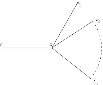
n > logM. Consider the
graph G on n+2 vertices (see Figure 3) which is defined as follows. The vertex set is{r,x, v1, . . . , vn}. There is an edge from r to x , and there is an edge from x
to each ofv1. . . vn. For convenience, define M = M/log n and N =n/log M.
Notice that the restriction we have placed onMimplies that N >
√ n.
The adversary operates in at most log N phases: we describe the i-th phase, 1≤ i ≤log N . In phase i the adversary divides the verticesv1. . . vn into classes
r x
v1
v2
[image:18.612.218.394.126.272.2]v n
Figure 3: The lower bound graph for Theorems 2 and 3
repeats the same process again. If requests have been generated at log M classes for the same multicast, the adversary moves on to the next multicast. At the end of all M multicasts for this phase, the adversary moves on to the next phase. Notice that setting the class size to 2i−1 is equivalent to doubling available profit by 2 for each phase.
Let c(i)be the capacity on the edge(r,x)used by the online algorithm during phase i. Also, let p(i) be the profit obtained by online during the i-th phase. Let p∗(i)and c∗(i) be the corresponding quantities for the solution generated by the oblivious adversary. Notice thatPic(i) can be at most 1. Define S(k) =
1 2k
P
1≤kE(p(i)). The total expected profit obtained by the algorithm in the first k
phases is 2kS(k).
We give brief proofs for the following two claims.
Claim 8.1 E(p(i)) <2iE(c(i)).
Proof: Suppose the online algorithm decides to satisfy a fractional demand of x for a specific multicast in the i-th phase. The cost incurred is x . Suppose that this commitment is made by the algorithm after the j -th request for this multi-cast group comes in. Then the expected profit from this multimulti-cast group is 2i−1· xPj≤j0≤M2j0−j < 2ix . Now we sum this up over all the multicast groups in phase i to get the desired result.
Claim 8.2 During any phase i, the adversary can ensure that
E(p∗(i))≥ log M 4 2
Proof: During phase i, the adversary can pick the multicast with the maximum number of classes of requests. Let P<(i) denote the probability of this number being less than i. Now, P<(i) = (1/2+1/4+. . .21−i)M = (1−21−i)M, for i <log M. Clearly, P<(23log M) < 1/3.3 This tells us that the expected number of classes is greater thanlog M2 . To complete the proof of this claim we observe that each class in the i-th phase has 2i−1requests.
We now prove that there exists a phase k such that the total expected profit ob-tained by the online algorithm during the first k phases is no more than 2k+1/log N . Suppose this is not true. Then, S(i) >2/log N for all i. In particular,
X
1≤i≤log N
S(i) >2.
But X
i
S(i)=X
i
E(p(i)) X
i≤j≤log N
1 2i ≤2
X
i
E(p(i))/2i.
Using Claim 8.1, we have X
i
E(c(i)) >1.
But this is a contradiction, as the online is not allowed to overflow capacities. This proves the existence of a phase k with S(k)≤2/log N .
The oblivious adversary cannot see the coin tosses of the online algorithm but it can compute in advance the quantities S(i). Having found the value k guaranteed by the above argument, the adversary stops after phase k and does not generate any more multicast requests. The adversary also generates a ‘good’ solution as follows: It does not satisfy any demands in the first k−1 phases, and in the last phase, it uses up the entire edge(r,x). Now from Claim 8.2, E(p∗(k)) ≥2k−2log M. The total expected profit obtained by the online algorithm is 2kS(k) ≤ 2k+1/log N . This gives a lower bound of(log M log N)on the competitive ratio of any online algorithm. Since N ≥√n and M =M/log n, this is also a(logMlog n)lower
bound.
In the above analysis, we assumed that√n >logM. This is not a very
restric-tive assumption, because for logM >
√
n, our proof shows that the competitive ratio is already as bad as(√n).
Now we adapt this lower bound proof to our model. Assume that the capacity is u. Let Mbe the number of multicasts, and let M
0 =
M/u. The adversary
3This is a very loose statement. P<(2
3log M)is much,much smaller, but we do not need a stronger
proceeds as before, except that each phase gets repeated u times. Also, the on-line algorithm is restricted to satisfy the entire demand of 1 unit or none at all. The same calculation as done above gives a lower bound of (logM0log n) =
(log(M/u)log n).
8.2
Against an adaptive-online adversary
Recall that an adaptive-online adversary is one which can adapt the input sequence depending on the response of the online algorithm; however the adversary must also generate a solution as it goes along.
Theorem 3 No randomized algorithm for selective online multicast can have bet-ter than(min(n,M
u )) competitive ratio against an adaptive-online adversary.
The lower bound holds even when the requests are non-interleaved.
Proof: Consider the same graph as in the previous section (see Figure 3). Each edge has a capacity u, all requests have demand 1. The value ofMis fixed at 2nu.
The adversary works in 2u phases.
During the i-th phase, the adversary chooses a number mi uniformly at random
from the set{1, . . . ,n}. The adversary then does the following for at most mi −1
sub-phases. It generates a new SET-UP request at r . It then generates, in sequence, requests at nodesv1, . . . , vn for the newly set up multicast group. As soon as the
online algorithm accepts any of these requests, the adversary aborts this phase com-pletely and moves to the next phase. If the online algorithm does not accept any of these n requests, the adversary moves to the next sub-phase. The adversary does not accept any request during the first mi −1 sub-phases. If all mi −1 sub-phases
end without the online algorithm having accepted even one request, then the ad-versary generates yet another SET-UP request at node r . It then generates requests in sequence at nodesv1, . . . , vn and accepts them all without bothering about the
online algorithm (if the edge< r,x >is already full in the adversary’s network, the adversary rejects these requests). During any phase, the online algorithm gets a profit of n if it ‘guesses’ correctly the value mi, and at most 1 otherwise. Since mi
is chosen uniformly at random from{1, . . . ,n}, the expected profit for the online algorithm during any one phase is at most 2.
References
[1] J. Aspnes, Y. Azar, A. Fiat, S. Plotkin, and O. Waarts. On-line load balancing with applications to machine scheduling and virtual circuit routing. 25th ACM Symposium on Theory of Computing, pages 623–31, 1993.
[2] B. Awerbuch, Y. Azar, A. Fiat, and T. Leighton. Making commitments in the face of uncertainty: How to pick a winner almost every time. 28th ACM Symposium on Theory of Computing, pages 519–530, 1996.
[3] B. Awerbuch, Y. Azar, and S. Plotkin. Throughput competitive online routing. 34th IEEE symposium on Foundations of Computer Science, pages 32–40, 1993.
[4] B. Awerbuch and T. Singh. Online algorithms for selective multicast and maximal dense trees. 29th ACM Symposium on Theory of Computing, 1997.
[5] N. Garg. A 3-approximation for the minimum tree spanning k vertices. 37th IEEE Symposium on Foundations of Computer Science, pages 302–309, 1996.
[6] A. Goel and S. Plotkin. An algorithm for throughput competitive online mul-ticasting in capacitated networks. Unpublished Manuscript.
[7] M. Goemans and J. Kleinberg. An improved approximation ratio for the min-imum latency problem. 7th ACM-SIAM Symposium on Discrete Algorithms, pages 152–158, 1996.
[8] M. Goemans and D. Williamson. A general approximation technique for constrained forest problems. SIAM J. Comput., 24(2):296–317, April 1995.
[9] A. Kamath, O. Palmon, and S. Plotkin. Routing and admission control in general topology networks with poisson arrivals. 7th ACM-SIAM Symposium on Discrete Algorithms, pages 269–278, 1996.
[10] J. Kleinberg and E. Tardos. Disjoint paths in densely embedded graphs. 36th IEEE symposium on Foundations of Computer Science, pages 52–61, 1995.
A
Making our algorithm run in polynomial time
There are two issues we need to address to make our algorithm run in polynomial time. First, in step 3 of VAi,j (Figure 1), we need to compute the minimum profit
needed out of the new request to create an appropriate tree fragment. Second, we need to provide a polynomial time approximation algorithm for finding the fragment in step 3 of VAi,j.
The first problem can be solved by doing a binary search. Letπbe the available profit on the node where the new request has been generated. We run a maximal dense tree algorithm with allπ units of profit available. If a non-empty tree is returned, we try with half the profit, and so on. The key observation here is that we can afford to incur an additive error of 1/(8n L)in finding the minimum profitπ0. Therefore, the binary search needs to be done only up to a depth log 8πn L. The competitive ratio remains unaffected by this modification.