A Hassle-Free Unsupervised Domain Adaptation Method
Using Instance Similarity Features
Jianfei Yu
School of Information Systems Singapore Management University
Jing Jiang
School of Information Systems Singapore Management University
Abstract
We present a simple yet effective unsu-pervised domain adaptation method that can be generally applied for different NLP tasks. Our method uses unlabeled tar-get domain instances to induce a set of instance similarity features. These fea-tures are then combined with the origi-nal features to represent labeled source do-main instances. Using three NLP tasks, we show that our method consistently out-performs a few baselines, including SCL, an existing general unsupervised domain adaptation method widely used in NLP. More importantly, our method is very easy to implement and incurs much less com-putational cost than SCL.
1 Introduction
Domain adaptation aims to use labeled data from a source domain to help build a system for a target domain, possibly with a small amount of labeled data from the target domain. The problem arises when the target domain has a different data distri-bution from the source domain, which is often the case. In NLP, domain adaptation has been well studied in recent years. Existing work has pro-posed both techniques designed for specific NLP tasks (Chan and Ng, 2007; Daume III and Ja-garlamudi, 2011; Yang et al., 2012; Plank and Moschitti, 2013; Hu et al., 2014; Nguyen et al., 2014; Nguyen and Grishman, 2014) and general approaches applicable to different tasks (Blitzer et al., 2006; Daum´e III, 2007; Jiang and Zhai, 2007; Dredze and Crammer, 2008; Titov, 2011). With the recent trend of applying deep learn-ing in NLP, deep learnlearn-ing-based domain adap-tation methods (Glorot et al., 2011; Chen et al., 2012; Yang and Eisenstein, 2014) have also been adopted for NLP tasks (Yang and Eisenstein, 2015).
There are generally two settings of domain adaptation. We usesupervised domain adaptation
to refer to the setting when a small amount of la-beled target data is available, and when no such data is available during training we call it unsu-pervised domain adaptation.
Although many domain adaptation methods have been proposed, for practitioners who wish to avoid implementing or tuning sophisticated or computationally expensive methods due to either lack of enough machine learning background or limited resources, simple approaches are often more attractive. A notable example is the frus-tratingly easy domain adaptation method proposed by Daum´e III (2007), which simply augments the feature space by duplicating features in a clever way. However, this method is only suit-able for supervised domain adaptation. A later semi-supervised version of this easy adaptation method uses unlabeled data from the target do-main (Daum´e III et al., 2010), but it still requires some labeled data from the target domain. In this paper, we propose a general unsupervised domain adaptation method that is almost equally hassle-free but does not use any labeled target data.
Our method uses a set of unlabeled target in-stances to induce a new feature space, which is then combined with the original feature space. We explain analytically why the new feature space may help domain adaptation. Using a few dif-ferent NLP tasks, we then empirically show that our method can indeed learn a better classifier for the target domain than a few baselines. In partic-ular, our method performs consistently better than or competitively with Structural Correspondence Learning (SCL) (Blitzer et al., 2006), a well-known unsupervised domain adaptation method in NLP. Furthermore, compared with SCL and other advanced methods such as the marginalized struc-tured dropout method (Yang and Eisenstein, 2014) and a recent feature embedding method (Yang and
Eisenstein, 2015), our method is much easier to implement.
In summary, our main contribution is a simple, effective and theoretically justifiable unsupervised domain adaptation method for NLP problems.
2 Adaptation with Similarity Features
We first introduce the necessary notation needed for presenting our method. Without loss of gen-erality, we assume a binary classification problem where each input is represented as a feature vec-tor xfrom an input vector space X and the out-put is a label y ∈ {0,1}. This assumption is general because many NLP tasks such as text cat-egorization, NER and relation extraction can be cast into classification problems and our discus-sion below can be easily extended to multi-class settings. We further assume that we have a set of labeled instances from a source domain, denoted byDs={(xs
i, yis)}Ni=1. We also have a set of un-labeled instances from a target domain, denoted by Dt = {xt
j}Mj=1. We assume a general setting of learning a linear classifier, which is essentially a weight vector w such that x is labeled as 1 if
w>x≥0.1
A naive method is to simply learn a classifier fromDs. The goal of unsupervised domain
adap-tation is to make use of bothDsandDt to learn a
goodwfor the target domain. It has to be assumed that the source and the target domains are similar enough such that adaptation is possible.
2.1 The Method
Our method works as follows. We first randomly select a subset of target instances from Dt and
normalize them. We refer to the resulting vectors asexemplar vectors, denoted byE = {e(k)}K
k=1. Next, we transform each source instance x into a new feature vector by computing its similarity with eache(k), as defined below:
g(x) = [s(x,e(1)), . . . , s(x,e(K))]>, (1)
where>indicates transpose ands(x,x0)is a
sim-ilarity function between x and x0. In our work
we use dot product as s.2 Once each labeled 1A bias feature that is always set to be 1 can be added to allow a non-zero threshold.
2We find that normalizing the exemplar vectors results in better performance empirically. On the other hand, if we nor-malize both the exemplar vectors and each instancex, i.e. if we use cosine similarity ass, the performance is similar to not normalizingx.
source domain instance is transformed into a K -dimensional vector by Equation 1, we can ap-pend this vector to the original feature vector of the source instance and use the combined feature vectors of all labeled source instances to train a classifier. To apply this classifier to the target do-main, each target instance also needs to add this K-dimensional induced feature vector.
It is worth noting that the exemplar vectors are randomly chosen from the available target in-stances and no special trick is needed. Overall, the method is fairly easy to implement, and yet as we will see in Section 3, it performs surpris-ingly well. We also want to point out that our in-stance similarity features bear strong similarity to what was proposed by Sun and Lam (2013), but their work addresses a completely different prob-lem and we developed our method independently of their work.
2.2 Justification
In this section, we provide some intuitive justifica-tion for our method without any theoretical proof.
Learning in the Target Subspace
Blitzer et al. (2011) pointed out that the hope of unsupervised domain adaptation is to “couple” the learning of weights for target-specific features with that of common features. We show our in-duced feature representation is exactly doing this. First, we review the claim by Blitzer et al. (2011). We note that although the input vector space X is typically high-dimensional for NLP tasks, the actual space where input vectors lie can have a lower dimension because of the strong fea-ture dependence we observe with NLP tasks. For example, binary features defined from the same feature template such as the previous word are mutually exclusive. Furthermore, the actual low-dimensional spaces for the source and the target domains are usually different because of domain-specific features and distributional difference be-tween the domains. Borrowing the notation used by Blitzer et al. (2011), define subspaceXs to be
the (lowest dimensional) subspace of X spanned by all source domain input vectors. Similarly, a subspace Xt can be defined. Define Xs,t =
XsTXt, the shared subspace between the two
do-mains. DefineXs,⊥to be the subspace that is
or-thogonal to Xs,t but together with Xs,t spans Xs,
that is,Xs,⊥+Xs,t =Xs. Similarly we can define
subspace and the domain-specific subspaces, and they are mutually orthogonal.
We can project any input vectorxinto the three subspaces defined above as follows:
x=xs,t+xs,⊥+x⊥,t.
Similarly, any linear classifier w can be decom-posed intows,t,ws,⊥andw⊥,t, and
w>x=w>
s,txs,t+w>s,⊥xs,⊥+w>⊥,tx⊥,t.
For a naive method that simply learnswfromDs,
the learned componentw⊥,twill be0, because the
componentx⊥,t of any source instance is0, and
therefore the training error would not be reduced by any non-zero w⊥,t. Moreover, any non-zero ws,⊥learned fromDswould not be useful for the
target domain because for all target instances we havexs,⊥=0. So for awlearned fromDs, only
its componentws,tis useful for domain transfer.
Blitzer et al. (2011) argues that with unlabeled target instances, we can hope to “couple” the learning ofw⊥,t with that ofws,t. We show that
if we use only our induced feature representation without appending it to the original feature vec-tor, we can achieve this. We first define a ma-trix ME whose column vectors are the exemplar
vectors from E. Then g(x) can be rewritten as M>
Ex. Let w0 denote a linear classifier learned
from the transformed labeled data. w0makes
pre-diction based onw0>M>
Ex, which is the same as
(MEw0)>x. This shows that the learned classifier w0for the induced features is equivalent to a linear
classifierw=MEw0for the original features.
It is not hard to see that MEw0 is essentially
P
kwk0e(k), i.e. a linear combination of vectors
inE. Becausee(k) comes fromX
t, we can write e(k)=e(k)
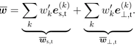
s,t +e(⊥,tk). Therefore we have
w=X
k
wk0e(s,tk)
| {z }
ws,t
+X
k
wk0e(⊥,tk)
| {z }
w⊥,t
.
There are two things to note from the formula above. (1) The learned classifierwdoes not have any component in the subspace Xs,⊥, which is
good because such a component would not be use-ful for the target domain. (2) The learnedw⊥,twill
unlikely be zero because its learning is “coupled” with the learning ofws,tthroughw0. In effect, we
pick up target specific features that correlate with useful common features.
In practice, however, we need to append the in-duced features to the original features to achieve good adaptation results. One may find this counter-intuitive because this results in an ex-panded instead of restricted hypothesis space. Our explanation is that because of the typicalL2 regu-larizer used during training, there is an incentive to shift the weight mass to the additional induced fea-tures. The need to combine the induced features with original features was also reported in previ-ous domain adaptation work such as SCL (Blitzer et al., 2006) and marginalized denoising autoen-coders (Chen et al., 2012).
Reduction of Domain Divergence
Another theory on domain adaptation developed by Ben-David et al. (2010) essentially states that we should use a hypothesis space that can achieve low error on the source domain while at the same time making it hard to separate source and tar-get instances. If we use only our induced fea-tures, then Xs,⊥ is excluded from the hypothesis
space. This is likely to make it harder to distin-guish source and target instances. To verify this, in Table 1 we show the following errors based on three feature representations: (1) The training error on the source domain (εˆs). (2) The
classi-fication error when we train a classifier to sepa-rate source and target instances. (3) The error on the target domain using the classifier trained from the source domain (εˆt). ISF- means only our
in-duced instance similarity features are used while ISF uses combined feature vectors. The results show that ISF achieves relatively low εˆs and
in-creases the domain separation error. These two factors lead to a reduction inεˆt.
features εˆs domain separation error εˆt
Original 0.000 0.011 0.283
ISF- 0.120 0.129 0.315
[image:3.595.115.249.590.637.2]ISF 0.006 0.062 0.254
Table 1:Three errors of different feature representations on a spam filtering task.Kis 200 for ISF- and ISF. We expect a lowεˆtwhenεˆsis low and domain separation error is high.
Difference from EA++
(2010). Here we briefly discuss how our method is different from EA++ in terms of using unla-beled data. In both EA and EA++, since launla-beled target data is available, the algorithms still learn two classifiers, one for each domain. In our al-gorithm, we only learn a single classifier using labeled data from the source domain. In EA++, unlabeled target data is used to construct a reg-ularizer that brings the two classifiers of the two domains closer. Specifically, the regularizer de-fines a penalty if the source classifier and the tar-get classifier make different predictions on an un-labeled target instance. However, with this regu-larizer, EA++ does not strictly restrict either the source classifier or the target classifier to lie in the target subspace Xt. In contrast, as we have
pointed out above, when only the induced features are used, our method leverages the unlabeled tar-get instances to force the learned classifier to lie in
Xt.
3 Experiments
3.1 Tasks and Data Sets
We consider the following NLP tasks.
Personalized Spam Filtering (Spam): The data set comes from ECML/PKDD 2006 discovery challenge. The goal is to adapt a spam filter trained on a common pool of 4000 labeled emails to three individual users’ personal inboxes, each contain-ing 2500 emails. We use bag-of-word features for this task, and we report classification accuracy.
Gene Name Recognition (NER): The data set comes from BioCreAtIvE Task 1B (Hirschman et al., 2005). It contains three sets of Medline ab-stracts with labeled gene names. Each set corre-sponds to a single species (fly, mouse or yeast). We consider domain adaptation from one species to another. We use standard NER features includ-ing words, POS tags, prefixes/suffixes and contex-tual features. We report F1 scores for this task.
Relation Extraction (Relation): We use the ACE2005 data where the annotated documents are from several different sources such as broadcast news and conversational telephone speech. We re-port the F1 scores of identifying the 7 major rela-tion types. We use standard features including en-tity types, enen-tity head words, contextual words and other syntactic features derived from parse trees.
3.2 Methods for Comparison Naiveuses the original features.
Common uses only features commonly seen in both domains.
SCL is our implementation of Structural Corre-spondence Learning (Blitzer et al., 2006). We set the number of induced features to 50 based on pre-liminary experiments. For pivot features, we fol-low the setting used by Blitzer et al. (2006) and se-lect the features with a term frequency more than 50 in both domains.
PCAuses principal component analysis onDt to
obtainK-dimensional induced feature vectors and then appends them to the original feature vectors.
ISF is our method using instance similarity fea-tures. We first transform each training instance to a K-dimensional vector according to Equation 1 and then append the vector to the original vector.
For all the three NLP tasks and the methods above that we compare, we employ the logistic re-gression (a.k.a. maximum entropy) classification algorithm with L2 regularization to train a clas-sifier, which means the loss function is the cross entropy error. We use the L-BFGS optimization algorithm to optimize our objective function.
3.3 Results
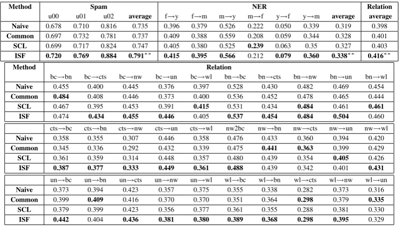
In Table 2, we show the comparison between our method and Naive, Common and SCL. For ISF, the parameter K is set to 100 for Spam, 50 for NER and 500 for Relation after tuning. As we can see from the table, Common, which removes source domain specific features during training, can sometimes improve the classification perfor-mance, but this is not consistent and the improve-ment is small. SCL can improve the performance in most settings for all three tasks, which confirms the general effectiveness of this method. For our method ISF, we can see that on average it outper-forms both Naive and SCL significantly. When we zoom into the different source-target domain pairs of the three tasks, we can see that ISF out-performs SCL in most of the cases. This shows that our method is competitive despite its simplic-ity. It is also worth pointing out that SCL incurs much more computational cost than ISF.
Method Spam NER Relation
u00 u01 u02 average f→y f→m m→y m→f y→f y→m average average Naive 0.678 0.710 0.816 0.735 0.396 0.379 0.526 0.222 0.050 0.339 0.319 0.398
Common 0.697 0.732 0.781 0.737 0.409 0.388 0.559 0.208 0.059 0.344 0.328 0.401
SCL 0.699 0.717 0.824 0.747 0.405 0.380 0.525 0.239 0.063 0.35 0.327 0.403
ISF 0.720 0.769 0.884 0.791∗∗ 0.415 0.395 0.566 0.212 0.079 0.360 0.338∗∗ 0.416∗∗
Method Relation
bc→bn bc→cts bc→nw bc→un bc→wl bn→bc bn→cts bn→nw bn→un bn→wl
Naive 0.455 0.400 0.445 0.376 0.397 0.528 0.430 0.482 0.469 0.454
Common 0.484 0.408 0.446 0.373 0.400 0.536 0.452 0.478 0.465 0.444
SCL 0.467 0.395 0.453 0.391 0.415 0.531 0.434 0.484 0.461 0.461 ISF 0.474 0.434 0.455 0.446 0.405 0.537 0.454 0.484 0.504 0.460 cts→bc cts→bn cts→nw cts→un cts→wl nw2bc nw→bn nw→cts nw→un nw→wl
Naive 0.358 0.355 0.307 0.446 0.358 0.476 0.433 0.360 0.394 0.420
Common 0.345 0.336 0.292 0.432 0.339 0.475 0.441 0.363 0.399 0.429
SCL 0.361 0.359 0.314 0.448 0.357 0.480 0.439 0.354 0.405 0.426
ISF 0.387 0.377 0.333 0.449 0.361 0.488 0.439 0.342 0.401 0.431
un→bc un→bn un→cts un→nw un→wl wl→bc wl→bn wl→cts wl→nw wl→un
Naive 0.373 0.394 0.423 0.357 0.375 0.355 0.338 0.282 0.373 0.316
Common 0.399 0.409 0.416 0.370 0.370 0.351 0.364 0.298 0.379 0.335 SCL 0.379 0.399 0.423 0.356 0.377 0.361 0.355 0.288 0.381 0.330
[image:5.595.99.499.61.288.2]ISF 0.442 0.404 0.436 0.381 0.380 0.389 0.368 0.298 0.395 0.329
Table 2: Comparison of performance on three NLP tasks. For each source-target pair of each task, the performance shown is the average of 5-fold cross validation. We also report the overall average performance for each task. We tested statistical significance only for the overall average performance and found that ISF was significantly better than both Naive and SCL with
p <0.05(indicated by∗∗) based on the Wilcoxon signed-rank test.
Method Spam
u00 u01 u02 average Naive 0.678 0.710 0.816 0.735
PCA 0.700 0.718 0.818 0.745
ISF 0.720 0.769 0.884 0.791∗∗
Table 3:Comparison between ISF and PCA.
4 Conclusions
We presented a hassle-free unsupervised domain adaptation method. The method is simple to im-plement, fast to run and yet effective for a few NLP tasks, outperforming SCL, a widely-used un-supervised domain adaptation method. We believe the proposed method can benefit a large number of practitioners who prefer simple methods than so-phisticated domain adaptation methods.
Acknowledgment
We would like to thank the reviewers for their valuable comments.
References
Shai Ben-David, John Blitzer, Koby Crammer, Alex Kulesza, Fernando Pereira, and Jennifer Wortman Vaughan. 2010. A theory of learning from
differ-ent domains. Machine Learning, 79(1-2):151–175.
John Blitzer, Ryan McDonald, and Fernando Pereira. 2006. Domain adaptation with structural
correspon-dence learning. In Proceedings of the 2006
Con-ference on Empirical Methods in Natural Language Processing, pages 120–128. Association for Com-putational Linguistics.
John Blitzer, Sham Kakade, and Dean P. Foster. 2011.
Domain adaptation with coupled subspaces. In
Pro-ceedings of the Fourteenth International Conference on Artificial Intelligence and Statistics, pages 173– 181.
Yee Seng Chan and Hwee Tou Ng. 2007. Domain adaptation with active learning for word sense
dis-ambiguation. In Proceedings of the 45th Annual
Meeting of the Association of Computational Lin-guistics, pages 49–56.
Minmin Chen, Zhixiang Eddie Xu, Kilian Q. Wein-berger, and Fei Sha. 2012. Marginalized denoising
autoencoders for domain adaptation. In
Proceed-ings of the 29th International Conference on Ma-chine Learning.
Hal Daume III and Jagadeesh Jagarlamudi. 2011. Do-main adaptation for machine translation by
min-ing unseen words. In Proceedings of the 49th
An-nual Meeting of the Association for Computational Linguistics: Human Language Technologies, pages 407–412.
Hal Daum´e III, Abhishek Kumar, and Avishek Saha. 2010. Frustratingly easy semi-supervised domain
adaptation. In Proceedings of the 2010 Workshop
on Domain Adaptation for Natural Language Pro-cessing, pages 53–59.
Hal Daum´e III. 2007. Frustratingly easy domain
[image:5.595.101.259.362.413.2]the Association of Computational Linguistics, pages 256–263.
Mark Dredze and Koby Crammer. 2008. Online meth-ods for multi-domain learning and adaptation. In
Proceedings of the Conference on Empirical Meth-ods in Natural Language Processing, pages 689– 697.
Xavier Glorot, Antoine Bordes, and Yoshua Bengio. 2011. Domain adaptation for large-scale sentiment
classification: A deep learning approach. InIn
Pro-ceedings of the Twenty-eight International Confer-ence on Machine Learning.
Lynette Hirschman, Marc Colosimo, Alexander Mor-gan, and Alexander Yeh. 2005. Overview of
BioCreAtIvE task 1B: normailized gene lists. BMC
Bioinformatics, 6(Suppl 1):S11.
Yuening Hu, Ke Zhai, Vladimir Eidelman, and Jordan Boyd-Graber. 2014. Polylingual tree-based topic
models for translation domain adaptation. In
Pro-ceedings of the 52nd Annual Meeting of the Asso-ciation for Computational Linguistics, pages 1166– 1176.
Jing Jiang and ChengXiang Zhai. 2007. Instance
weighting for domain adaptation in nlp. In
Proceed-ings of the 45th Annual Meeting of the Association of Computational Linguistics, pages 264–271. Abhishek Kumar, Avishek Saha, and Hal Daume.
2010. Co-regularization based semi-supervised
do-main adaptation. InAdvances in neural information
processing systems, pages 478–486.
Thien Huu Nguyen and Ralph Grishman. 2014. Em-ploying word representations and regularization for
domain adaptation of relation extraction. In
Pro-ceedings of the 52nd Annual Meeting of the Asso-ciation for Computational Linguistics, pages 68–74. Minh Luan Nguyen, Ivor W. Tsang, Kian Ming A. Chai, and Hai Leong Chieu. 2014. Robust domain adaptation for relation extraction via clustering
con-sistency. InProceedings of the 52nd Annual
Meet-ing of the Association for Computational LMeet-inguis-
Linguis-tics, pages 807–817.
Barbara Plank and Alessandro Moschitti. 2013. Em-bedding semantic similarity in tree kernels for
do-main adaptation of relation extraction. In
Proceed-ings of the 51st Annual Meeting of the Association for Computational Linguistics, pages 1498–1507. Chensheng Sun and Kin-Man Lam. 2013.
Multiple-kernel, multiple-instance similarity features for
effi-cient visual object detection. IEEE Transactions on
Image Processing, 22(8):3050–3061.
Ivan Titov. 2011. Domain adaptation by constraining inter-domain variability of latent feature
representa-tion. InProceedings of the 49th Annual Meeting of
the Association for Computational Linguistics: Hu-man Language Technologies, pages 62–71.
Yi Yang and Jacob Eisenstein. 2014. Fast easy unsu-pervised domain adaptation with marginalized
struc-tured dropout. In Proceedings of the 52nd Annual
Meeting of the Association for Computational Lin-guistics, pages 538–544.
Yi Yang and Jacob Eisenstein. 2015. Unsupervised multi-domain adaptation with feature embeddings. InProceedings of the North American Chapter of the Association for Computational Linguistics, pages 672–682.
Pei Yang, Wei Gao, Qi Tan, and Kam-Fai Wong.
2012. Information-theoretic multi-view domain
adaptation. InProceedings of the 50th Annual
Meet-ing of the Association for Computational LMeet-inguis-