doi:10.4236/ijcns.2010.38086 Published Online August 2010 (http://www.SciRP.org/journal/ijcns)
Potential Vulnerability of Encrypted Messages:
Decomposability of Discrete Logarithm Problems
Boris S. Verkhovs ky
Computer Science Department, New Jersey Institute of Technology, Newark, USA E-mail: [email protected]
Received May 10, 2010; revised June 15, 2010; accepted July 21, 2010
Abstract
This paper provides a framework that reduces the computational complexity of the discrete logarithm prob-lem. The paper describes how to decompose the initial DLP onto several DLPs of smaller dimensions. De-composability of the DLP is an indicator of potential vulnerability of encrypted messages transmitted via open channels of the Internet or within corporate networks. Several numerical examples illustrate the frame- work and show its computational efficiency.
Keywords:Network Vulnerability, System Security, Discrete Logarithm, Integer Factorization, Multi-Level Decomposition, Complexity Analysis
1. Introduction
and Problem Statement
The cryptoimmunity of numerous public key cryptogra- phic protocols is based on the computational complexity of the discrete logarithm problems [1,2].
A DLP finds an integer x satisfying the equation
mod x
g p=h. (1) Here 2≤ ≤ −g p 1; 1≤ ≤ −h p 1 (2) and p is a large prime. In (1) g, p and h are inputs, and the unknown integer x must be selected on the interval
[
1,p−1]
.Two trivial cases: if h = 1, then x = p – 1; If h = g, then x = 1. If h is neither 1 nor g, then x must be selected on the interval [2, p – 2].
If g is a generator, then (1) always has a solution, oth-erwise the existence of a solution is not guaranteed.
For instance, if p = 7 and g = 2, then the DLP 2 mod 7x =5
does not have a solution.
Various algorithms for solving the DLP were proposed and their computational complexities were analyzed over the last forty years [3-15].
This paper provides the algorithmic framework that reduces the computational complexity of the DLP.
The paper describes step-by-step procedure for deco- mposition of the initial DLP onto several DLPs with smaller dimensions. Several examples illustrate the dec- omposition algorithm and highlight its computational efficiency.
Let g1:=g h; 1:=h x; 1:=x;
1: 1
q = −p and p− =1 2r r1 2. (3)
Here it is assumed that integer factors r1 and r2 in (3)
are known or can be determined using existing algo-rithms for integer factorization [5,16,17].
Proposition: Let R1:=
(
p−1 /)
q; (4) if q|(
p−1)
, then R1 is an integer (4).Let’s define 1
2: 1 mod
R
g =g p; (5)
1
2: 1 mod
R
h =h p; (6) If an integer x2 is a solution of equation
2
2 mod 2
x
g p=h , where x2∈
[ ]
0,q , (7)then q divides x1−x2.
Proof: Let’s multiply both sides of the Equation (1) by
2
1 mod
x
g− p [18], and find x2, such that
2
1 1 mod
x
h g− p (8) has a root of power q.
By Euler’s criterion [5] such a root exists if and only if
(
)
( )2 1 /
1 1 mod 1
p q
x
h g− − p= (9)
Using notations (4)-(6), rewrite (8) as
2
2 2 mod 1
x
h g − p= (10)
Therefore, the unknown x1 can be represented as
1 2 3
x =x +qx (11) where the integer x3 must be on the interval
[
]
[
]
3 0, ( 1) / 0, 3
x ∈ p− q = q (12)
After x2 is determined, we need to find an integer
3
x , for which the following equation holds
2 3
1 mod 1
x qx
g + p=h. (13)
This equation can be rewritten as
( )
3 2(
)
1 1 1 mod
x x
q
g =h g− p (14)
where in contrast with the BSGS algorithm, the value of
2
x is already known.
Let ( 1 /) 3
3: 1 mod
p q
g =g − p; (15)
and 2
3: 1 1 mod
x
h =h g− p. (16)
2. Divide-and-Conquer Decomposition:
Illustrative Example-1
Let’s solve 2 mod947 273x1 = , (17)
i.e., here g1=2;p=947;h1=273, and x1∈
[
1, 946]
.Let q1:= −p 1.
Sinceq1=2r r1 2 = × ×2 11 43, select
(
)
2 min0 z p1max ,( 1)/ 43
q = ≤ ≤ − z p− z = .
ThenR1:=q1/q2=22; 1
22
2: 1 mod 2 mod 947
R
g =g p=
41
= ; and 1 22
2: 1 mod 273 mod 947 283
R
h =h p= = .
Therefore we need to solve the DLP(2):
2
41 mod 947x =283 (7), (18) where x2∈
[
1, 42]
.Remark1: Notice that the interval of uncertainty [1, 42] for x2 is much smaller than the corresponding interval
of uncertainty [1, 946] for x1.
Equation (18) can be solved using any algorithm for the DLP [3,6,8-10,12].
In this example x2 = 39 and q2=43.
Therefore x1=39 43+ x3, where
(
)
[
]
3 0, 1 / 2 0, 22
x ∈ p− q = .
To find x3 solve the DLP(3):
( )
43 3 39(
)
2 x =273 2× − mod 947 , which is equivalent to
(
)
3
367x =273 111× =946 mod 947 . (19) Therefore x3 =11.
Verification: 11
367 mod 947=946. (20) Finally, x1=39 43 11+ × =512.
3. Multi-Level Decomposition: Illustrative
Example-2
Initial DLP(1): Find an integer x1, such that
1
30 mod 99991x =45636
, (21)
where x1∈
[
1, 99990]
.Because 99990=303*330, select q2 =330 and
represent the unknown x1 as x1=x2+330x3.
Since R1:=
(
p−1 /)
q2 =303;then 303
2: 1 mod 99991 151
g =g = ;
and h2:=h1303mod 99991=64099.
Remark2: To better describe the concept of decompo-sition, a more suitable system of notations is considered below in the following Table1. These notations are used to describe the process of solving three DLPs.
DLP(2): Solve 2
2 mod 99991 2
x
g =h ,
i.e., 151 mod 99991x2 =64099,
where x2∈
[
0, 330]
. (22)The solution is x2 =115; indeed
115
151 mod 99991=64099.
Therefore 30x1 =30115 330+ x3mod 99991=45636.
Consider the equation
(
330)
3 115(
)
30 x =30− ×45636 mod 99991 . Let g3: 30= 330mod 99991= 2593; and
(
)
115 3
115
: 30 45636
96658 45636 mod 99991
49845
h = − ×
= ×
=
Therefore, we need to solve
DLP(3): 2593 mod 99991x3 =49845, where
[
]
3 0, 303
x ∈ . (23)
It is easy to verify that x3=47. Finally,
1 2
x =x +q x2 3=115 330 47+ × =15625.
Decomposition of DLP(2): Solve 2
2 mod 2
x
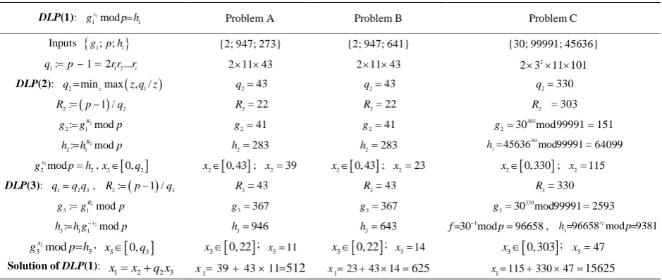
641 Table 1. Solutions of DLP(1) via the decomposition of DLP(2) and DLP(3).
DLP(1): 1 1 mod 1
x
g p h= Problem A Problem B Problem C
Inputs {g1; ;p h1} {2; 947; 273} {2; 947; 641} {30; 99991; 45636}
1: 1 21 2...t
q =p− = r r r 2 11 43× × 2 11 43× × 2
2 3× × ×11 101
DLP(2): q2=min maxz (z q z, 1/ ) q2= 43 q2= 43 q2= 330
( )
2: 1 / 2
R = p− q R2= 22 R2= 22 R2 = 303
2 2: 1 mod
R
g =g p g2=41 g2=41
303
2 30 mod99991 151
g = =
2 2: 1 mod
R
h =h p h2=283 h2=283
303 2 45636 mod99991
h= = 64099
2 2mod 2
x
g p=h,x2∈[0,q2] x2∈[0, 43]; x2=39 x2∈[0, 43]; x2=23 x2∈[0, 330]; x2=115 DLP(3): q1=q q2 3, R3:=(p−1 /) q3 R3= 43 R3= 43 R3= 330
3 3: 1 mod
R
g =g p g3=367 g3=367
330
3 30 mod99991 2593
g = =
2 3: 1 1 mod
x
h =h g− p h3=946 h3=643
1
30 mod 96658
f= − p= , 2
3 96658 mod 9381
x
h= p=
3
3 mod 3 x
g p h= ,
[
]
3 0, 3
x ∈ q x3∈
[
0, 22]
; x3=11 x3∈[
0, 22]
; x3=14 x3∈[
0, 303]
; x3=47 Solution of DLP(1):1 2 2 3
x =x +q x x1=39+43× =11 512 x1=23+43 14× =625 x1=115+330×47=15625
Remark3: Notice that the interval of uncertainty in DLP(2) is not [1, p – 1], but x2∈
[
1,q2]
, which is muchsmaller than [1, p – 1].
Instead of solving (24) directly using an existing DLP algorithm, we can again apply the method of decomposi-tion described above. Consider a factor q4 of q2 that
is close to the square root of q2= 330:
(
)
(
)
2
4 min0 max , 2/
min max , 330 / 30
z q
z
q z q z
z z
≤ ≤ =
= = (25)
Let’s represent the unknown in (24) as
2 4 4 5
x =x +q x , (26)
[
] [
]
[
] [ ]
4 4
5 5 2 4
where 1, 1, 30
and 1, : / 1,11
x q
x q q q
∈ =
∈ = = . (27)
Let us now investigate whether h2 has an integer
root of power 30 modulo p.
By Euler’s criterion, such a root exists if and only if ( 1 /) 4
2 mod 1
p q
h − p= . (28)
However, if ( 1 /) 4
2 mod 1
p q
h − p≠ , find an integer x4, which satisfies the equation
(
)
( ) 44 1 /
2 2 mod 1
p q
x
h g− − p= . (29)
Let ( 1 /) 4
4: 2 mod
p q
g =g − p; (30)
and ( 1 /) 4
4: 2 mod
p q
h =h − p. (31)
Now we need to solve the equation
4
4 mod 4
x
g p=h , (32) where x4∈
[
0, 30]
. And again, the Equation (32) itself isalso a DLP with a much smaller interval (27) for x4 than
the interval for x2 in (24), and so on.
4. Multi-Level Decomposition: Illustrative
Example-3
First level: Let’s solve the equation 1
1 mod 1
x
g p=h, where
g = 2, p = 4,000,000,003,231; and h = 3,024,336,139,227. Then p – 1 = 863*2310*2006491, where 863 and 2,006,491 are primes.
In this case the initial DLP(1) 1
1 mod 1
x
g p=h ; is
de-composable into two sub-problems: DLP(2) and DLP(3).
DLP(2): Compute ( 1 /) 2 2 1
1993530
:
2 mod 4000000003231
p q
g =g −
=
=3278213345371; and ( 1 /) 2
2: 1
p q
h =h −
=30243361392271993530 mod 4000000003231 =2084778340641.
Solve 2
2 mod 4000000003231 2
x
g =h , where
2 2
0≤x ≤q =2006491; It is easy to verify the solution
2 1853979 2006491
x = ≤ .
DLP(3):Compute
( 1 /) 3 2006491
3: 1 2 mod 4000000003231
p q
g =g − =
2 3 1 1
1853979 3024336139227 2000000001616
mod 4000000003231
:
3024336139227 629308445687
mod4000000003231
2623468766941.
x
h h g−
×
=
= ⋅
= × ⋅
=
Solve 3
(
)
3 3 mod
x
g =h p , where
(
)
3 3 2
0≤x =14622≤q = p−1 /q =1993530; and q1=q q2 3.
Then
1 2 2 3
=1,853, 979 2, 006, 491 14, 622 =29, 340, 765, 381.
x x q x
∗
= + +
It is easy to verify that the solution
3 14622 1993530
x = ≤ .
Comparison of complexities: While the size of the required memory/storage for DLP(1) equals
1 1 2000000
T = p− = ;
the corresponding memory requirement for DLP(2) and DLP(3) are respectively
2 2 1 2006491 1416
T = q − = =
and T3= q3−1 = 1993530=1411.
Therefore the speed-up ratio
(
)
(
)
1/ 2 3 2000000 / 1416 1411 707.
S=T T +T = + =
Thus the decomposition algorithm for solving DLP(1) via DLP(2) and DLP(3) is 707 times faster than a direct solution of the original DLP(1).
5. Second-Level Decomposition: Solution of
DLP(3)
Remark4: The second problem, DLP(2), cannot be sol- ved by decomposition since q2 = 2,006,491 is a prime integer. However, the third problem, DLP(3), is decom-posable, therefore the speed-up ratio S can be further increased.
Indeed, select
(
)
3
6: min0 z q max 3/ ,
q = ≤ ≤ q z z = 2310.
Let’s represent x3 as x3=x6+q x6 7, where
6 6
0<x <q =2310 and 0<x7<q7 =863,
and solve DLP(3) by decomposition into DLP(6) and DLP(7).
DLP(6): Compute ( 1 /) 6
6: 3 mod
p q
g =g − p;
and ( 1 /) 6
6: 3 mod
p q
h =h − p;
where q q6 7=q3=1993530;
and solve 6
(
)
6 6 mod1993531
x
g =h ;
{0<x6<q6=2310}.
DLP(7): Compute ( 1 /) 7
7: 3 mod
p q
g =g − p;
and 6
7: 3 3 mod
x
h =h g− p;
and solve 7
(
)
7 7 mod1993531
x
g =h ;
{0<x7<q7=863}.
Then T6= q6=48 and T7= q7=29.
Therefore
(
)
(
)
1/ 2 6 7
=2000000/ 1416 48 29 =2000000/1493
= ,
S =T T + +T T
+ +
1339.6
which implies that by decomposing the original problem DLP(1) into three sub-problems {DLP(2), DLP(6) and DLP(7)}, we can solve the initial DLP(1) 1340 times faster than if we directly solve it without employing de-composition.
In general, the speed-up increases as the size of p in-creases.
6. Computational Considerations
It is quite reasonable to ask under what conditions should we stop the decomposition of a DLP(k) and try to solve it directly. Here are the major issues that must be taken into the consideration:
1) Feasibility of factoring qk=q q2k 2k+1 in such a way
that
( 1 /) 2
2 : mod 1
k
p q
k k
g =g − p≠ ± . (33)
For instance, if q q2 4| 2
(
p−1)
, then( ) ( ) ( )
( ) ( )
(
)
4
4 2
2 4
1 /
1 / 1 /
4 2 1
1 / 2
2 1 /
1
:
1 mod
p q
p q p q
p
p q q
w w w
w p
−
− −
− −
= =
= = ± , (34)
where w = {g, h}. In such a case Equation (32) has only trivial solutions {0 or 1} or no solution
if g4=1 and h4= −1.
2) Magnitude of the overhead computations required to find g2k and g2k+1 and then to solve these two DLPs,
643
become too “costly”.
Remark 4: Analogously, we can solve DLP(3) by de-composing it into two DLPs with smaller intervals of uncertainty for the corresponding unknowns.
7. Algorithmic Decomposition of DLP(k)
Suppose that we need to solve DLP(k)
mod
k
u
k k
g p=h , (33) where uk∈
[
0,qk]
.If qk is a prime or if factors of qk are unknown, then (33) can be solved by an algorithm for DLP such as: BSGS, Pollard’s rho-algorithm, Lenstra’s number field algorithm etc. However, if qk =cd, where both c and d are integers, then the DLP(k) can be reduced to solving two less complex DLPs: DLP(2k) and DLP(2k + 1).
Let qk =q q2k 2k+1;
DLP(2k): Solve 2
2 mod 2
k
u
k k
g p=h ; (34) where q2k :=c and u2k∈
[ ]
0,c ; (35)(
)
: 1 /
k k
R = p− q ; (36)
2 : mod
k
R
k k
g =g p; (37) and 2 : Rk mod
k k
h =h p; (38)
DLP(2k+1): Solve
2 1
2 1 mod 2 1
k
u
k k
g + p h
+ = + ; (39)
where u2k+1∈
[
0,qk/c]
, (40)(
)
2k 1: 1 / 2k 1
R + = p− q + ; (41)
2 1
2 1: k mod
R
k k
g g + p
+ = ; (42)
and 2
2 1: kmod
u
k k k
h + =h g− p. (43)
8. Conclusions
Provided that we know how to factor p – 1, we can reduce the initial DLP(1) to two discrete logarithm problems: DLP(2) and DLP(3), for solution of which the best known algorithms can be implemented. The decomposition can be implemented recursively for solution of the DLP(k) by reducing it to a pair of DLP(2k) and DLP(2k + 1).
9. Acknowledgements
I express my appreciation to R. Rubino and P. Fay for their comments and suggestions that improved the style of this paper.
10. References
[1] W. Diffie and M. E. Hellman, “New Directions in Cry- ptography,” IEEE Transactions on Information Theory, Vol. 22, No. 6, 1976, pp. 644-654.
[2] T. ElGamal, “A Public Key Cryptosystem and a Digital Signature Scheme Based on Discrete Logarithms,” IEEE
Transactions on Information Theory, Vol. 31, No. 4, 1985,
pp. 469-472.
[3] L. M. Adleman and J. DeMarrais, “A Sub-Exponential Algorithm for Discrete Logarithms over all Finite Fields,”
Mathematics of Computation, Vol. 61, No. 203, 1993, pp.
1-15.
[4] E. Bach, “Discrete Logarithms and Factoring,” Technical
Report: CSD-84-186, University of California, Berkeley,
1984.
[5] R. Crandall and C. Pomerance, “Prime Numbers: A Com- putational Perspective,” The Quadratic Sieve Factorization
Method, Springer, Berlin, 2001, pp. 227- 244.
[6] A. Enge and P. Gaudry, “A General Framework for Sub- Exponential Discrete Logarithm Algorithms,” Research
Report LIX/RR/00/04, Luxembourg Internet eXchange
(LIX), Luxembourg Kirchberg, Vol. 102, June 2000, pp. 83-103.
[7] B. A. LaMacchia and A. M. Odlyzko, “Computation of Discrete Logarithms in Prime Fields,” Designs, Codes
and Cryptography, Vol. 19, No. 1, 1991, pp. 47-62.
[8] A. K. Lenstra and J. H. W. Lenstra, “The Development of the Number Field Sieve,” Lecture Notes in Mathematics, Springer-Verlag, Berlin, Vol. 1554, 1993, pp. 95-102. [9] V. Müller, A. Stein and C. Thiel, “Computing Discrete
Logarithms in Real Quadratic Congruence Function Fie- lds of Large Genus,” Mathematics of Computation, Vol. 68, No. 226, 1999, pp. 807-822.
[10] O. Schirokauer, “Using Number Fields to Compute Log- arithms in Finite Fields,” Mathematics of Computation, Vol. 69, No. 231, 2000, pp. 1267-1283.
[11] D. Shanks, “Class Number, a Theory of Factorization and Genera,” Proceedings of Symposium in Pure Mathematics, Vol. 20, American Mathematical Society, Providence, 1971, pp. 415-440.
[12] J. Silverman, “The xedni Calculus and the Elliptic Curve Discrete Logarithm Problem,” Designs, Codes and
Cryp-tography, Vol. 20, No. 1, 2000, pp. 5-40.
[13] D. C. Terr, “A Modification of Shanks’ Baby-Step Giant- Step Algorithm,” Mathematics of Computation, Vol. 69, No. 230, 2000, pp. 767-773.
[14] B. Verkhovsky, “Generalized Baby-Step Giant-Step Alg- orithm for Discrete Logarithm Problem,” Advances in
Decision Technology and Intelligent Information Systems,
International Institute for Advanced Studies in Systems Research and Cybernetics, Baden-Baden, 2008, pp. 88- 89.
ANTS-III, Lecture Notes in Computer Science, Springer, Berlin, Vol. 1423,1998, pp. 621-638.
[16] J. P. Pollard, “A Monte Carlo Method for Factorization,”
BIT Numerical Mathematics, Vol. 15, No. 3, 1975, pp.
331-334.
[17] C. Pomerance, J. W. Smith and R. Tuler, “A Pipeline Architecture for Factoring Large Integerswith the
Qua-dratic Sieve Algorithm,” SIAM Journal on Computing, Vol. 17, No. 2, 1988, pp. 387-403.
[18] B. Verkhovsky, “Multiplicative Inverse Algorithm and its Complexity,” Proceedings of International Conference
on System Research, Informatics & Cybernetics, Baden-
Baden, 28-30 July 1999, pp. 62-67.
APPENDIX
Numeric example as an exercise
Let p = 5,000,491; then p− =1 990 5051× Let
1 2 and 1 1020305
g = h = .
In this case DLP(1) is 2x1=1020305 mod 5000491
(
)
,where the unknown x1∈
[
1,p−1]
.The DLP(1) is decomposable into two sub-problems:
DLP(2): 2
(
)
2 2 mod
x
g =h p {see (4)-(6)}, where
[
] [
]
2 1, 2 1, 5051
x ∈ q =
;
and DLP(3): 3
(
)
3 3 mod
x
g =h p {see (15) and (16)},
where
[ ] [
]
3 1, 3 1, 990
x ∈ q =
. Therefore x1=x2+q x2 3.
Remark5: The reader now has an opportunity to solve this problem himself since values required for the de-composition are purposely omitted.
From DLP(2) and DLP(3) we find that
2 1947 5051
x = < ;
and x3=470<990. Finally,
1 1947 5051 470 2375917.
x = + × =