Yu He,1, 2X. Ding,1, 2 Z.-E. Su,1, 2H.-L. Huang,1, 2J. Qin,1, 2 C. Wang,1, 2 S. Unsleber,3 C. Chen,1, 2H. Wang,1, 2Y.-M. He,1, 3 X.-L. Wang,1, 2W.-J. Zhang,4S.-J. Chen,4 C. Schneider,3
M. Kamp,3 L.-X. You,4 Z. Wang,4S. H¨ofling,1, 3, 5 Chao-Yang Lu,1, 2and Jian-Wei Pan1, 2 1Hefei National Laboratory for Physical Sciences at Microscale and Department of Modern Physics,
University of Science and Technology of China, Hefei, Anhui 230026, China
2
CAS-Alibaba Quantum Computing Laboratory, CAS Center for Excellence in Quantum Information and Quantum Physics, University of Science and Technology of China, China
3
Technische Physik, Physikalisches Instit¨at and Wilhelm Conrad R¨ontgen-Center for Complex Material Systems, Universitat W¨urzburg, Am Hubland, D-97074 W¨uzburg, Germany
4
State Key Laboratory of Functional Materials for Informatics, Shanghai Institute of Microsystem and Information Technology (SIMIT), Chinese Academy of Sciences, 865 Changning Rd., Shanghai 200050, China
5
SUPA, School of Physics and Astronomy, University of St. Andrews, St. Andrews KY16 9SS, United Kingdom (Dated: April 19, 2017)
Boson sampling is a problem strongly believed to be intractable for classical computers, but can be naturally solved on a specialized photonic quantum simulator. Here, we implement the first time-bin-encoded boson sam-pling using a highly indistinguishable (∼94%) single-photon source based on a single quantum-dot-micropillar device. The protocol requires only one single-photon source, two detectors and a loop-based interferometer for arbitrary number of photons. The single-photon pulse train is time-bin encoded and deterministically injected into an electrically programmable multi-mode network. The observed three- and four-photon boson sampling rates are 18.8 Hz and 0.2 Hz respectively, which are more than 100 times faster than previous experiments based on parametric down-conversion.
Boson samping, proposed by Aaronson and Arkhipov [1], has received considerable interest as a model of non-universal (intermediate) quantum computation that can outperform clas-sical computers. It is a sampling task that can be carried out by sendingnindistinguishable single photons to am-mode (m>n) optical interferometer, and measure the output photon number distribution. boson sampling doesn’t require adaptive measurement, deterministic entangling gates, and makes less stringent demands on device performance than universal opti-cal quantum computing [2].
Previous work [3–7] have demonstrated the working princi-ple of boson sampling using pseudo-single photons produced by spontaneous parametric down-conversion (SPDC) [8]. An intrinsic problem in the SPDC, however, is that the photon pairs are generated probabilistically, and mixed with double pair emission. To overcome this problem, protocols of scat-tershot boson sampling [9] and spatial/temporal multiplexing [10, 11] were proposed to enhance the multi-photon coun-t racoun-te. Yecoun-t, so far coun-the boson sampling experimencoun-ts based on SPDC were limited up to three single-photon Fock states for arbitrary input configurations.
To scale up to a larger number of photons and fast sampling rate, a more efficient route is to use single-photon sources that emit one and only one photon each time [12–14]. To be useful for multi-photon interference, the photons should simultane-ously fulfill a checklist that include high system efficiency, near-perfect purity and indistingushability [15]. The single-photon system efficiency (η) can be calculated as the number of single photons output from a single-mode fiber divided by the pulsed laser repetition rate. It would be affected by the quantum efficiency of the emitter, population inversion
effi-ciency, extraction effieffi-ciency, and loss in the optical path. For n-photon boson sampling, the finaln-fold coincidence rate is proportional toηn. The photon purity can be characterized by second-order correlationg2(τ), which givesg2(0)=0for an ideal single-photon source with no multi-photon mixture. The photon indistinguishability can be quantified by the visibili-ty of two-photon Hong-Ou-Mandel interference. High levels of photon purity and indistinguishability are key prerequisites for the boson sampling to be a classically intractable problem [16–18]. Recently, by pulseds-shell resonant excitation [19] of a single quantum dot (QD) embedded in a micropillar, these criteria have been compatibly combined [15, 20, 21].
For n-photon boson sampling, the most straightforward method is to usenseparate QDs that emit transform-limited s-ingle photons at the same wavelength. This is still challenging due to the inhomogeneity of self-assembled QDs [22] and less perfect two-photon interference from independent QDs [23]. A unique solution is based on only one single-photon emit-ter, which is more resource efficient. An additional advan-tage of this approach is that for single photons from the same QD with emission time separated by less than∼1µs—shorter than the time scale of spectral wandering—their mutual indis-tinguishability is protected in a subspace and remains close to unity [20]. Here, we demonstrate boson sampling with a single-photon device, where the photons are time-bin encod-ed and interferencod-ed in an electrically programmable multi-mode network in a loop-based architecture [24–26]. Such a setup also allows us to track the dynamical evolution step-by-step inside the optical circuit.
single-(b)
(c)
b
in n
u
m
b
e
r
1 2 3
Loop
1
2
3
4
4 ....
M
N
[image:2.612.72.550.54.276.2](a)
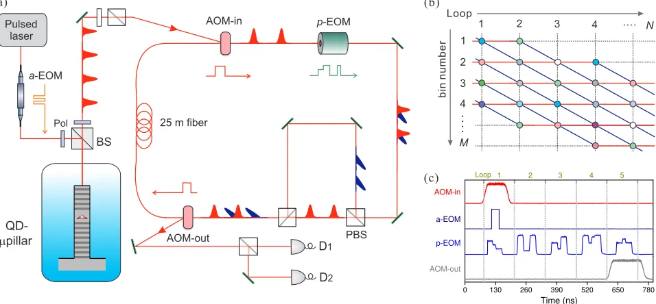
FIG. 1. Boson sampling with a single-photon device. (a) Experimental arrangement. The pumping laser is chopped by a waveguide-based amplitude electro-optic modulator (a-EOM) to prepare a single-photon pulse train in designed time bins. The QD is sandwiched between 25.5 lower and 15 upperλ/4-thick AlAs/GaAs mirror pairs that form distributed Bragg reflectors, and embedded inside a 2.5µm diameter micropillar. The device is cooled to 7 K where the QD emission is resonant with the micropillar cavity mode. A confocal microscope is utilized to address the QD, and laser leakage is extingushed by applying cross-polarizers on its both arms. The prepared three or four single photons are injected into a loop by an acousto-optic modulator (AOM). An electro-optical modulator (p-EOM) rotates the polarization controlled by a pulse sequence. The red (blue) pulse in the loop denotes horizontal (vertical) polarization. A 25 m single-mode fiber is used to increase the loop length to 130 ns (10 bins). After several loops of evolution (see text for details), the photons are ejected out of the loop by the AOM-out and detected with two superconducting nanowire single-photon detectors. (b) An equivalent beam splitter network unravelling the dynamics ofM time bins circulating forNloops. The circles denote beam splitter operations and their color coding represents arbitrary, electrically programmable coupling ratios. The red and blue line evolution represents the trajectory for horizontal and vertical polarization, respectively. (c) Electrical pulse sequences for implementing Boson sampling. The whole system is time synchronized to the pulsed laser.
mode fiber, of which 12.9 MHz are eventually detected by a superconducting nanowire single-photon detectors with an efficiency of 52% and a dead time of less than 13 ns (see Fig. 1(a) and Supplemental Materials [27] for more details). Such a single-photon source is∼10 times more efficient than the state-of-the-art SPDC [28]. Second-order correlation of 0.027(1) is observed at zero time delay, proving the highly pu-rified single-photon Fock state. Thanks to thes-shell resonant excitation that eliminates dephasings and emission time jitter, we observe two-photon interference visibilities of 0.939(3) for two photons with their emission time separated by 13 ns.
To implement the multi-mode interferometer, we utilize a scalable time-bin encoding scheme [24–26], as illustrated in Fig. 1(a). For each experimental period, M time bins (each loaded with one or zero photon) are injected into a loop by an acousto-optical mudulator (AOM) and circulated forNloops. Such a loop-based architecture is equivalent to anM-mode beam splitter network with a depth of N, as illustrated in Fig. 1(b). Here, the polarization degree of freedom acts as the spatial mode in the conventional boson sampling model. The beam splitter operations, denoted by the circles in Fig. 1(b), are effectively realized using a polarization-rotation electro-optic modulator (p-EOM) with dynamically programmable coupling ratio. After the p-EOM, a polarization-dependent
asymmetric Mach-Zehnder interferometer delays the vertical polarization for one time-bin length (∼13 ns), regarding to the horizontal polarization, which realizes the displacement oper-ation of the time bins.
AfterN loops of evolution, theM bins are ejected out of the loop by another AOM, and the output distribution are ob-tained by registering all the single-photon detection events in real time and postprocessing [27]. In this experimen-t, the optical transmission efficiency per loop is 83.4%, and the injection and extraction efficiency in each AOM is 85%. We calibrate the mode matching of the time-bin loop using Mach-Zehnder interference, and we obtain an interference visibility of 99.5%. The time-bin encoding scheme natural-ly complements the single-photon pulse train. We note that the loop-based architecture is intrinsically stable, electrical-ly programmable, and resource efficient. For an arbitrary n-boson sampling, this scheme requires only one single-photon emitter, two optical switches, two EOMs, and two fast de-tectors, whereas the traditional spatial-encoding approach re-quiresn−1 optical switches, ∼n4beam splitters, and∼n2
detectors [27]. Furthermore, it relaxes the overhead of active-ly demultiplexing a single photon source [29] or building an array of multiple identical single photon sources [22].
20 output distributions, from (1,2,3), (1,2,4), ... to (4,5,6)
p-EOM
p-EOM
[image:3.612.61.558.49.251.2]70 output distributions, from (1,2,3,4), (1,2,3,5), ... to (5,6,7,8) 1 2 3 4 5 6 7 8 1 2 3 5 6 4 7 8 0.9 0.4 0.7 0.4 0.5 0.5 0.5 0.3 0.5 0.6 0.6 0.5 0.6 0.3 0.1 0.2 0.6 0.1 0.4 0.6 0.7 0.1 0.3 0.1 0.6 1 2 3 4 5 6 1 2 3 4 5 6 0.3 0.5 0.7 0.9 0.3 0.6 0.6 0.8 0.6 0.2 0.2 0.9 0.6 (a) (b) (c) (d)
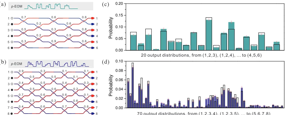
FIG. 2. Experimental results for 3- and 4-boson sampling. (a), (b) The equivalent 3- and 4-boson sampling circuits implemented. The upper panel shows the electrical pulse sequence that drives thep-EOM and programs the circuits. The inputs to the circuits are one (zero) photon Fock state, represented by solid (empty) circles. (c), (d) The measured relative frequencies of various output combinations, denoted by (i,j,k) wherei,j, andkare the output modes as labelled in (a) and (b). The solid bars indicates the normalized coincidence rate for different output distribution. The empty bars are theoretical calculations in the ideal case. The error bar represents one standard deviation from Poissonian counting statistics.
0 1000 2000 3000 4000 5000 6000 -20
-10 0 10 20
1 10 100
0.0 0.5 1.0
[image:3.612.64.554.342.483.2]0 1000 2000 3000 4000 5000 6000 -40 -20 0 20 40 3 4 3 4 uniform sampler A A c o u n te r ( × 1 0 2 ) Events boson sampler (c) (b) mean-field sampler boson sampler 3 4 3 4 B a y e s ia n c o u n te r Events (a) distinguishable sampler 3 4 3 4 L R c o u n te r ( × 1 0 2 ) Events boson sampler
FIG. 3. Validating boson sampling results. Solid lines are tests applied on the experimental data. Dotted lines are tests applied on simulated data generated from the three alternative hypotheses. The counter is updated every single event and a positive value indicates the data is obtained from a genuine boson sampler. Red lines are results for 3 bosons and blue lines are for 4 bosons. (a) Using the Aaronson and Arkhipov (AA) test to rule out the uniform distribution. (b) The Bayesian analysis is applied to ditinguish from mean-field distribution. (c) Standard liklihood ratio test is applied to discriminate the data from a distinguishable sampler.
photons, propagating them through the loop-based interfer-ometers withm=6 andm=8 modes forN=5 andN=7 loops, respectively. Figure 2(a) and 2(b) show two typical equiva-lent boson sampling circuits, programmed by electric pulse sequences shown in the upper panels that drive the p-EOM [27]. We measure no-collision (one photon per output-mode) coincidence events of 20 and 70 different combinations of out-put distributions for the 3- and 4-boson sampling, respective-ly. A total of 5626 and 5372 events are recorded in the 3-and 4-boson sampling within 5 minutes 3-and 7.6 hours, respec-tively. The high-efficiency single-photon source allows us to run the 3-boson sampling∼100 times faster than the best
pre-vious work with SPDC [3–7]. The experimental probability distributions (solid bar) are shown in Fig. 2(c)-(d) with theo-retically evaluated distributions (empty bars) through caculat-ing the permanent of the correspondcaculat-ing submatrix. To make a comparsion between the normalized distributions obtained experimentally (qi) and theoretically (pi), the measure of the
fidelity: F=P i
√
piqi is applied. From the data shown in
1st loop 2nd loop 3rd loop 4th loop 5th loop
[image:4.612.66.553.51.240.2](a) (b) (c) (d) (e)
FIG. 4. Tracking boson sampling dynamics. The output distribution is measured after 1 (a), 2 (b), 3 (c), 4 (d), and 5 (e) loops evolution in the 3-boson sampling circuit shown in Fig. 2(a). The probability of finding three photons in the output-mode distributions (i,j,k) (see Fig. 2 caption) are plotted using a sphere centered at coordinates (i,j,k), where the volume of the sphere is proportional to the occurring frequency. The measured fidelities from the 1st to the 5th loop are 0.981(6), 0.985(0), 0.991(2), 0.967(2), and 0.993(2), respectively. The upper and lower panels are the experimental data and theoretical calculation, respectively.
As the boson sampling is related to a problem strongly be-lieved to be in the #P-complete complexity class, not only the calculation but also a full certification of its outcome could be-come exponentially intractable for classical computation. To this end, there have been proposals [31–33] and demonstra-tions [34, 35] for validation of boson sampling, and discrim-inate the genuie boson sampling result with some other type-s of type-sampling hypothetype-sitype-s. Firtype-stly, we apply the experimen-tal data to the Aaronson and Arkhipov test [31], designed to distinguish the outcome of fixed-input boson sampling from a uniform distribution (see Fig. 3(a)). In our test, the uni-form distribution can be conclusively ruled out with ∼200 events. Secondly, we employ the Bayesian analysis [32] to exclude the possibilities of a mean-field sampler [36] (see Fig. 3(b)). With only∼15 events, a confidence level of 99.8% is achieved, proving that the output distribution data are from a genuine boson sampler. Finally, we adapt the standard like-lihood ratio test [33, 35] to rule out the hypothesis that the data could be reproduced with a sampler with distinguishable bosons. Fig. 3(c) shows an increasing discrepancy between indistingushable photons (solid lines) and distingushable pho-tons (dotted lines) against the increase of sampling events, and confirms that our data are indeed expected from highly indis-tinguishable single photons.
The flexible loop-based architecture in this experiment fur-ther allow us to track the dynamical multi-photon evolution in the circuit at intermediate time. Controlled by the ejection time of the AOM-out (Fig. 1a), the output distribution can be measured and monitored, on a loop-by-loop basis. The evolu-tion of the multi-photon scattering of a new 3-boson sampling circuit (supplementary information) at the end of the 1-5 loop are shown in Fig. 4(a)-(e), respectively. The measured fideli-ties (upper panels) from the 1st to the 5th loop are 0.981(6),
0.985(0), 0.991(2), 0.967(2), and 0.993(2), respectively, in a good agreement with the theoretical calculations (lower pan-els). Our experiment opens a new way to study multi-particle high-dimensional quantum walks with single quantum emit-ters [26, 37, 38]. We also anticipate that our platform would be useful for other applications of boson sampling, such as sub-shotnoise quantum metrology [39].
The overall efficiency of the current experiment is mainly limited by the system efficiency of the single-photon source (∼24.7%, due to losses in light extraction, cross polariza-tion, optical path transmission, and fiber coupling), transmis-sion of the loop-based interferometer (∼83.4% per loop), and single-photon detection efficiency (∼52%). With on-going technological advances on deterministic QD-micropillar [40], background-free laser excitation (to avoid cross-polarization) [41], and high-efficiency superconducting nanowire single-photon detection [42, 43], boson sampling with rapidly in-creasing number of photons can be expected. Our work opens up a new avenue to multi-photon quantum computation with single quantum emitters, and brings boson sampling closer to an experimental regime approaching quantum supremacy.
After the first version of our experiment was complete [44], we became aware of a related work on 3-boson sampling us-ing passively demultiplexed sus-ingle-photon source from a non-resonantly pumped QD [45].
[1] S. Aaronson and A. Arkhipov, in Proceedings of the 43rd An-nual ACM Symposium on Theory of Computing (eds Fortnow, L.& Vadhan, S.), 333 (ACM Press, 2011).
[3] M. A. Broome, A. Fedrizzi, S. Rahimi-Keshari, J. Dove, S. Aaronson, T. C. Ralph, and A. G. White, Science339, 794 (2013).
[4] J. B. Springet al., Science339, 798 (2013).
[5] M. Tillmann, B. Daki´c, R. Heilmann, S. Nolte, A. Szameit, and P. Walther, Nat. Photon.7, 540 (2013).
[6] A. Crespiet al., Nat. Photon.7, 545 (2013).
[7] M. Bentivegnaet al.Science Advances1, e1400255 (2015). [8] P. G. Kwait, K. Mattle, H. Weinfurter, A. Zeilinger, A. V.
Sergienko, and Y. Shih, Phys. Rev. Lett.75, 4337 (1995). [9] A. P. Lund, A. Laing, S. Rahimi-Keshari, T. Rudolph, J. L.
O’Brien, T. C. Ralph, Phys. Rev. Lett.113, 100502 (2014). [10] T. B. Pittman, B. C. Jacobs, and J. D. Franson, Phys. Rev. A66,
042303 (2002).
[11] F. Kanedaet al.Optica2, 1010 (2015). C. Xionget al, Nat. Comm.7, 10853 (2016).
[12] P. Michler, A. Kiraz, C. Becher, W. V. Schoenfeld, P. M. Petroff, L. Zhang, E. Hu, and A. Imamo˘glu, Science290, 2282 (2000). [13] C. Santori, D. Fattal, J. Vu˘ckovi´c, G. S. Solomon, and Y.
Ya-mamoto, Nature419, 594 (2002).
[14] I. Aharonovich, D. Englund, and M. Toth, Nature Photonics10, 631 (2016)
[15] X. Ding, Y. He, Z.-C. Duan, N. Gregersen, M.-C. Chen, S. Un-sleber, S. Maier, C. Schneider, M. Kamp, S. H¨ofling, C.-Y. Lu, and J.-W. Pan, Phys. Rev. Lett.116, 020401 (2016).
[16] M. Tillmann, S.-H. Tan, S. E. Stoeckl, B. C. Sanders, H. de Guise, R. Heilmann, S. Nolte, A. Szameit, and P. Walther, Phys. Rev. X5, 041015 (2015).
[17] V. S. Shchesnovich, Phys. Rev. A91, 013844 (2015). [18] M. C. Tichy, Phys. Rev. A91, 022316 (2015).
[19] Y.-M. He, Y. He, Y.-J. Wei, D. Wu, M. Atat¨ure, C. Schneider, S. H¨ofling, M. Kamp, C.-Y. Lu, and J.-W. Pan, Nat. Nanotech.
8, 213 (2013).
[20] H. Wanget al., Phys. Rev. Lett.116, 213601 (2016). [21] J. C. Loredoet al.Optica3, 433 (2016).
[22] R. B. Patel, A. J. Bennett, I. Farrer, C. A. Nicoll, D. A. Ritchie, and A. J. Shields, Nat. Photonics4, 632 (2010).
[23] Y. He, Y.-M. He, Y.-J. Wei, X. Jiang, M.-C. Chen, F.-L. Xiong, Y. Zhao, C. Schneider, M. Kamp, S. H¨ofling, C.-Y. Lu, and J.-W. Pan, Phys. Rev. Lett.111, 237403 (2013).
[24] K. R. Motes, A. Gilchrist, J. P. Dowling, and P. P. Rohde, Phys. Rev. Lett.113, 120501 (2014).
[25] P. C. Humphreys, B. J. Metcalf, J. B. Spring, M. Moore, X.-M. Jin, M. Barbieri, W. S. Kolthammer, and I. A. Walmsley, Phys. Rev. Lett.111, 150501 (2013).
[26] A. Schreiber, K. N. Cassemiro, V. Potoˇcek, A. G´abris, P. J. Mosley, E. Andersson, I. Jex, and Ch. Silberhorn, Phys. Rev. Lett.104, 050502 (2010).
[27] see Supplemental Materials for more details.
[28] X.-L. Wanget al., Phys. Rev. Lett.117, 210502 (2016). [29] H. Wanget al.arXiv:1612.06956 (2016); F. Lenziniet al.
arX-iv:1611.02294 (2016).
[30] K. R. Motes, J. P. Dowling, A. Gilchrist, P. P. Rohde, Phys. Rev. A92, 052319 (2015)
[31] S. Aaronson and A. Arkhipov, Quant. Inf. Comp. 14, 1383 (2014).
[32] M. Bentivegnaet al., Int. J. Quant. Inf.12, 1560028 (2014). [33] T. M. Cover and J. A. Thomas, in Elements of Information
The-ory 2nd edn, (Wiley-Interscience, 2006). [34] J. Carolanet al., Nat. Photon.8, 621 (2014). [35] N. Spagnoloet al.Nat. Photon.8, 615 (2014).
[36] M. C. Tichy, K. Mayer, A. Buchleitner, and K. Mølmer, Phys. Rev. Lett.113, 020502 (2014).
[37] A. Peruzzo,et al.Science329, 1500 (2010).
[38] A. Schreiber, A. G´abris, P. P. Rohde, K. Laiho, M. ˇStefaˇn´ak, V. Potoˇcek, G. Hamilton, I. Jex, and C. Silberhorn, Science336, 55 (2012).
[39] K. R. Motes, J. P. Olson, E. Rabeaux, J. P. Dowling, S. J. Olson, and P. P. Rohde. Phys. Rev. Lett.114, 170802 (2015).
[40] S. Unsleber, Y.-M. He, S. Gerhardt, S. Maier, C.-Y. Lu, J.-W. Pan, N. Gregersen, M. Kamp, C. Schneider, and S. H¨ofling, Opt. Exp.24, 8539 (2016).
[41] E. B. Flagg, A. Muller, J. W. Robertson, S. Founta, D. G. Deppe, M. Xiao, W. Ma, G. J. Salamo, and C. K. Shih, Nat. Phys.5, 203 (2009).
[42] W.-J. Zhanget al.IEEE Photon. J.8, 2 (2016).
[43] I. E. Zadeh, J. W.N. Los, R. B.M. Gourgues, V. Steinmetz, S. M. Dobrovolskiy, V. Zwiller, S. N. Dorenbos, Preprint at http://arxiv.org/abs/1611.02726 (2016).
[44] Y. Heet al.arXiv:1603.04127.
[45] J. C. Loredo, M. A. Broome, P. Hilarie, O. Gazzano, I. Sagnes, A. Lemaitre, M. P. Almeida, P. Senellart, A. G. White, Phys. Rev. Lett.118, 130503 (2017).