doi:10.4236/ica.2011.23024 Published Online August 2011 (http://www.SciRP.org/journal/ica)
Autonomous Target Interception Using Hybrid Sensor
Networks*
Wenzhe Zhang1, Yihuai Wang1, Ying Li1, Minglu Li2
1
School of Computer Science and Technology, Soochow University, Soochow, China
2
Department of Computer Science and Engineering, Shanghai Jiaotong University, Shanghai, China E-mail: [email protected]
Received December 2, 2010; revised May 20, 2011; accepted May 27,2011
Abstract
Hybrid sensor networks (HSNs) comprise of mobile and static sensor nodes setup for purpose of collabora-tively performing tasks like sensing a phenomenon or monitoring a region. In this paper, we present target interception as a novel application using mobile sensor nodes as executor. Static sensor nodes sense, com-pute and communicate with each other for navigation. Mobile nodes are guided to intercept target by the static nodes nearby. Our approach does not require any prior maps of the environment thus, cutting down the cost of the overall energy consumption. As to multi-targets multi-mobile nodes case, we present a PMB al-gorithm for task assignment. Simulation results have verified the feasibility and effectiveness of our ap-proach proposed.
Keywords:Target, Hybrid Sensor Networks, Interception, CoS, Intercepting Strategy, PMB Task Assignment
1. Introduction
A networked system of hybrid sensor networks opens new frontiers in variety of civilian and military applica-tions and in some scientific disciplines. A mixture of networked mobile robots and static sensors reduce the cost but preserves the flexibility and advantageous capa-bilities of a multi-robot system.
We are broadly interested in the mutually beneficial collaboration between mobile and static sensor networks. The underlying principle in this hybrid network between the mobile and static nodes is that: the static nodes serve as the sensing, computation and communication medium, whereas the robots provide action and finish the task of blocking with the help of static sensors. In this work we describe results from such a system which accurately and reliably solves the problem of target interception. Some properties of our approach are summarized below:
1) The sensor network is pre-deployed into the envi-ronment deterministically or randomly for the full cov-erage of the region.
2) After deployment, static sensor nodes can sense the
condition of its environment. By the multi-hop commu-nication, static nodes compute the distributions of local environment and evaluate appearance of the target.
3) The nodes of the sensor network are synchronized in time (high precision is not required).
4) The mobile node is made up of a static sensor and a robot, so it can communicate with any static nodes nearby.
5) The environment is not required to be static. Sensor networks are deployed in the field of interest. They are expected to monitor the field and intercept any intruding target as soon as possible in an unmanned manner[1]. The concept of artificial potential fields for the purpose of obstacle avoidance was presented in [2-6]. The concept of Vector Field Histograms (VFH) based on locally constructed polar histograms for robot navigation was presented in [7]. It may be noted that a parallel ap-proach for the construction of a navigation field has been proposed in sensor network. It uses potential fields and the hop count to compute the magnitude of the direc-tional vectors. In our paper, we only use the static node nearby to guide the mobile node, which cut down the complication of computation greatly.
*This paper is supported by the Natural Science Foundation of China, No. 61070169, National Basic Research Program of China, No. 2006
strategy to address the problem of target interception. i.e.
When the target intrudes the sensory field, static sensor nodes that detect the events collectively elect one head that has sensed the largest intensity of signal. After data computing, it will generate a sensing report and flood over the network by multi-hops. We call the sensing re-port data stimulus and the head node as center of stimu-lus. Mobile sensor node acquires the position of target and decides its optimal pursuit direction with the help of sensors nearby. When the target moves, center of stimu-lus is re-elected and static sensor node keeps the proper position of the target. Only if the update of the network is enough, can the mobile node select its optimal strategy to intercept the target. Instead of a mobile node wander-ing randomly, in sign-based approach each static node decides the direction to guide the mobile node. As a re-sult, our approach with refreshing stimulus packets adapts to the mobile target, and can guide the mobile node to block the target as soon as possible.
We rely on the communication network to establish the navigation paths. Also, in our approach the mobile robots only need a local sense of target in order to move toward the correct direction. The obvious merit is that the mobile node does not need a pre-decided environ-ment map, or a compass.
The rest of the paper is organized as follows: We pre-sent sensing model, stimulus election and target localiza-tion in Seclocaliza-tion 2 Mobile node navigalocaliza-tion is presented in Section 3. In Section 4 we extend the case to multiple targets and mobile nodes and design the task assignment algorithms. Section 5 presents the simulation and evalu-ates its performance. Section 6 summarizes the work and sketches out our future plan.
2. Sensor Network Surveillance
2.1. Sensing Model
Let Ns be the number of static senor nodes, deployed
over the surveillance region R 2. Let
i
s R be the location of the i-th sensor node and let
i s . Let
i N
:1
S s G
S E,
be acommunica-tion graph such that s si, j E if and only if node i
can communicate with node j. Let m be the
number of mobile nodes (for simplicity,
s
N N
1
m
N ) and Let s be the sensing range of each static/mobile
sensor node. If there is a target at
R
xR, the sensor node can detect the presence of the target. Each sensor records the sensor’s signal strength,
1 i i i
i
i i
w if s x R
s x
S
w if s x
where , and are constants specific to the sen-sor type and they are normalized such that i has the
standard Gaussian distribution. This signal-strength based sensor model is general for sensors available in sensor networks, such as acoustic and magnetic sensors, and has been used frequently [8-10]. For each sensori, if
i
w
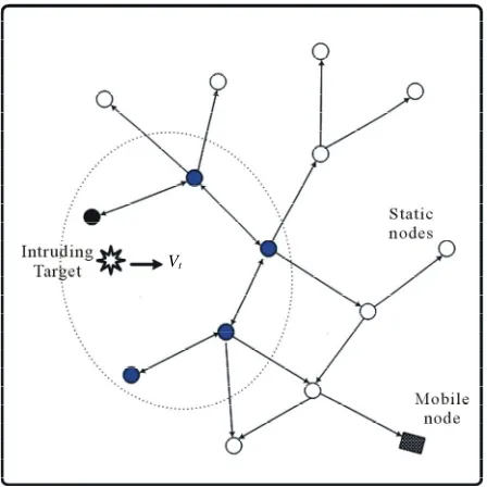
S , where is a threshold set for appropriate val-ues of detection and false-positive probabilities, the node is activated and join in the mesh as shown in Figure 1. It will participate in the stimulus election in the next sec-tion and may transmit its to its neighboring nodes if necessary.
i
S
2.2. Stimulus Election and Its Update
The election of a source follows the mechanism bellow. We want only one node to generate the report since it would be a waste of resources if every node detecting the target sends a report. The target creates a field of sensing signal strength, the nearer the sensor is, the signal strength it collects is larger.
Each node broadcasts a message indicating its signal strength and Cartesian coordinate (with some random delay to avoid collision). A node rebroadcasts its signal strength whenever it hears a neighbor’s message with a weaker signal, but stops broadcasting when it hears a stronger one. In this way, messages roll throughout the whole network of the signal strength field. Finally the node with the strongest signal is elected as the Center of Stimulus (CoS) and generates the sensing reports.
[image:2.595.312.536.449.673.2]Vt
Figure 1. The stimulus starts from a source and ends at the mobile node. The black nodes forward the packet to the source collectively. Notice that some nodes outside of the mesh also receive the packet but do not forward it.
s
s
R
2.3. Target Localization and Velocity Estimation
Computation of target’s information is performed by the node CoS. Let xi be the Cartesian coordinate of
sen-sor , the position of a target is estimated as i
1
1 *
ˆ j j
j
k i i j
i k
i j
S x
x
S
(2)then ˆxi is broadcasted as stimulus data all through the
network. In this way, although each sensor cannot give an accurate estimate of target’s position, as more sensors collaborate, the accuracy of estimates improves [11].
We assume mobile sensor node can move at some cer-tain velocity, here we note it as m. Target may intrude
into the monitoring region and move with the speed of maximum .
v
t
Based on the target location, we can calculate the ve-locity of the moving target as well. For simplicity, sup-pose the estimated positions of target at time 1and
2 are
v
t t xˆ1
x y1, 1
and xˆ2
x y2, 2
respectively, thevelocity of the target is computed as:
2
21 2 1 2
1 2
ˆt x x y y
v
t t
(3)
And the direction of velocity t:xˆ1xˆ2.
3. Mobile Node Navigation
3.1. Interception Strategy
We suppose the mobile node moves at a constant speed. In order to intercept the intruding target as soon as possi-ble, we need select the optimal direction of movement
m
according to the instant target. The target may in-trude the field of interest at any time with the velocity of
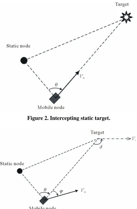
. At first, we consider the case of static target,
i.e. . As to the static target, the optimal strategy is intercepting towards the target as shown in Figure 2. So the intercept strategy is computed as:
max tv v
0
t
v
t
2 2 2
arccos 2
SM MT TS m
SM MT
d d d
d d
(4)
where are Euclidean distances of Static node-Mobile node, Mobile node-Target and Target-Sta- tic node.
, ,
SM MT TS
d d d
As to the mobile target, interception strategy needs modified according to the update of target’s position and velocity. Based on the velocity estimation in Section 2C, the additional offset of interception direction is computed as:
arcsin t sin
m
m
v v
m
(5)
So the optimal strategy of mobile target interception is computed as shown in Figure 3:
m m
(6)
3.2. Target Intercepting
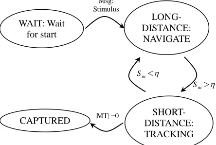
[image:3.595.312.534.361.698.2]During the interception performance, there are four states for mobile sensor node, i.e. WAIT, LONG-DISTANCE: NAVIGATE, SHORT-DISTANCE: TRACKING and INTERCEPTED. In the beginning there is no target in-truding into the region, so mobile node is waiting for a command, maybe wandering randomly. When the target appears in the region, CoS node injects the stimulus packet into the sensor network and activates the compu-tation to the position and velocity of the target. Receiv-ing the stimulus Message, mobile node come to the LONG-DISTANCE state and begins to navigate with the guidance of static node nearby. When the sensor of mo-bile node receives enough signal strength (above ), it
Figure 2. Intercepting static target.
will track the target in the current direction. Finally if the position and velocity of mobile node is the same with that of target, mission is completed. Note that when the signal strength received is less than the threshold, mo-bile node’s state will transit from SHOT-DISTANCE to LONG-DISTANCE, and come back to navigate with the help o f static nodes as shown in Figure 4.
3.3. Metrics of Interception
In the mission of target interception, several criteria may be chosen to evaluate the performance, such as minimi-zation of mobile node’s energy while guaranteeing cap-ture of all targets or maximization of number of capcap-tured targets within a certain amount of time. In this work we focus on minimizing the Time-to-Interception (TI) of mobile node. Since target’s motion is not known, exact TI is not known either; therefore we need to define a metric to estimate TI. We will use the following defini-tion of TI:
Definition 1. Let
p tt
0 ,v tt 0
2t
2
the posi-tion and velocity of a target at time t0 , and
22t t t
0 0 the position and velocity of a mobile node at time 1 0. We define the mini-mum time TI necessary for the mobile node to reach the target with the same velocity, assuming that the target will keep moving with constant velocity, i.e.,
,
m m
p t v t
1 1 1 1
min t m , t m
T
TI
T p t T p t T v t T v t T
where
1
0 1 0
* 0 , 1
t t
p t T p t t T t v t v t T v t0 . This definition allows us to quantify TI in an unambi-guous way. Although target can change trajectories over time, it is a more accurate estimate than, for example, some metric based on the distance between the target and
WAIT: Wait for start LONG- DISTANCE: NAVIGATE Msg: Stimulus SHORT- DISTANCE: TRACKING m
S <
CAPTURED |MT| =0
m
[image:4.595.59.281.550.699.2]S >
Figure 4. States transition diagram of mobile node.
the mobile node, since TI incorporates the dynamics of mobile node. Moreover, it is well-defined for any arbi-trary time delay td t1 t0 in the estimate of target’s position and velocity relative to current time 1. Given this definition and the constraints on the dynamics of the mobile node, it is possible to calculate explicitly TI.
t
4. Task Assignment Algorithms
In the previous section, we presented mobile sensor node interception and its metric for an intercepting pair. In this section we consider the case of multiple targets and mo-bile nodes. Given positions and velocities of all targets and mobile nodes, it is possible to compute TI matrix
,
m t
N N i j
Cc
c
, where m and t are the total
number of mobile nodes and targets, respectively, and the entry i j, of the matrix C corresponds to the ex-pected TI between mobile node i and target j. When co-ordinating multiple mobile nodes to intercept multiple targets, it is necessary to select an assignment. Our ob-jective is to select an assignment that minimizes the ex-pected TI of all mobile nodes.
N N
Assume that we have the same number of mobile nodes and targets, i.e. . An assignment can be represented as a matrix ,
m
N Nt
m t N N i j
X x , where the entry xi j, of the matrix X is equal to 1 if mobile node i is assigned to target j, and equal to 0 otherwise. The as-signment problem can therefore be written formally as follows:
,
, , 0,1 , 1, ,
, ,
1 1
min max
subject to 1, 1.
i j
i j i j x i j N
N N
i j i j
i j c x x x
(7)As formulated in the equation above, the assignment problem appears as a combinatorial problem.
One simple greedy assignment algorithm that tries to solve the optimization problem above is to look for the smallest TI entry in the matrix C, assign the correspond-ing interception pair, and remove the correspondcorrespond-ing row and column from the matrix C which now becomes of dimension
N 1
N1
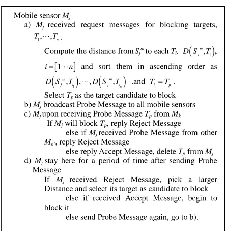
, and repeat the same process until each mobile node is assigned to a target. Although it is straightforward and easy to implement, this is a suboptimal algorithm, since there are cases when the greedy assignment gives the worst solution.In this section we present a collaborative task assign-ment protocol as Figure 5. The protocol assigns the task based on probe message in a distributed manner. Previ-ous work [11-13] gives a hierarchical multiple task as-signment protocol for the similar problem. But all of them are not distributed and is not scalable well.
Mobile sensor Mj
a) Mj received request messages for blocking targets,
1, , n
TT,
Compute the distance fromSjmto each Ti,
,
m
j i
D S T ,
1
i n and sort them in ascending order as
, 1
, ,
, n
m m
j i j i
D S T D S T .and
1
i p
T T .
Select Tp as the target candidate to block
b) Mj broadcast Probe Message to all mobile sensors
c) Mj upon receiving Probe Message Tp from Mk
If Mj will block Tp, reply Reject Message
else if Mj received Probe Message from other
Mk’, reply Reject Message
else reply Accept Message, delete Tp from Mj
d) Mj stay here for a period of time after sending Probe
Message
If Mj received Reject Message, pick a larger
Distance and select its target as candidate to block else if received Accept Message, begin to block it
[image:5.595.310.534.67.261.2]else send Probe Message again, go to b).
Figure 5. Pseudo-code of probe message based distributed task assignment.
multiple target and multiple mobile nodes, stimulus as-signs every target to one mobile node randomly in spite of negotiation among nodes. We will compare PMB al-gorithm with RTA in the latter simulation program.
5. Experimental Results
In order to gain a better understanding of landmark- based target interception, we have performed a wide range of simulation studies. In this section, we present several interesting results and discuss their implications and possible applications.
The main simulation platform is written in C++. The visualization and user interface elements are currently implemented with Visual C++ and OpenGL libraries. Network Simulator (ns2) and CrossBow® MICAZ sen-sor nodes are also used to verify the sensing models and the qualitative performance of the exposure model in a realistic environment. The sensor field in our experi-ments is defined as a 500 * 500 square. 80 static nodes are randomly deployed in the region.
For simplicity, parameters t and t is set to 0 and
respectively. Suppose a target intrudes from a point of the left edge and monitored by the networked sensors. The mobile node starts interception from the midpoint of the right edge. As shown in Figure 6, we calculate the intercepting path with m of 10 unit/s and 8 unit/s
re-spectively. And the velocity of the target is 6 unit/s.
v
max
t
v
v
max
t
v
If the target intrudes the field from different points, mobile node needs different time for interception. In-truding point of target has a great impact on the per-
10
m
v
8
m
[image:5.595.61.282.73.300.2]v
Figure 6. Intercepting paths with different speed vm.
formance of algorithms. We conducted 50 independent trials and the outcome is averaged.
The mobile node is deployed over the field randomly. When the target intrudes the field of interest from the left edge with 0, 100, 200, 300, 400 and 500 units, TI for target interception is shown in Figure 7. From Figure 7, we can conclude that TI is largest when the target in-trudes along the upper boundary (i.e. 0 unit) or bottom boundary (i.e. 500 units). This is because the mobile node is deployed randomly over the field of interest. When the target intrudes the field along the upper or bottom boundary, the relative distance between the target and the mobile node is the largest, so it needs the largest TI for interception. On the contrary, if the target intrudes from the midline point (i.e. 300 units), TI for interception is smaller.
The mobile node waits for the stimulus for intercep-tion from the original posiintercep-tion and begins to intercept the target. The original position has important impact on the
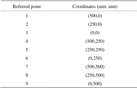
[image:5.595.315.535.535.703.2]TI. We build Cartesian coordinate in the monitored re-gion with the upper-left point as original point. And we select 9 referred points as the start point of the mobile node (See Table 1). Intruding point of the target is se-lected randomly from the left boundary and we con-ducted 50 independent trials. The average of TI is shown in Figure 8. From Figure 8, we can see that the mobile node needs least time for interception when starting from the referred point 5, i.e. TI of the mobile node from the center point of the monitored region is the smallest. So we can conclude that the center point of the region is the best guard point for the mobile node and the referred points of 1 and 7 are the worst.
In order to validate the effectiveness of PMB multiple task assignment, we conducted simulation as follows. Suppose the number of the targets is equal to that of the mobile nodes, i.e. m t . Velocity of all targets
is 6 unit/s and velocity of all mobile nodes is 8 unit/s. All mobile nodes are deployed over the field randomly and all targets intrude the field from the random point of the left edge. We conducted 50 independent trials and the outcome is averaged. TI changes with the number of targets N as shown in Figure 9. From Figure 9, we can see that TI of PMB algorithm reduces with the number of targets/ mobile nodes N grows, while TI of RTA algo-rithm almost holds the line. Besides, the advantage of PMB algorithm appears more distinctly when N grows. With the number of targets N growing, TI of PMB algo-rithm decrease more slowly. It can be explained by the fact that TI is mainly determined by the distance between the entry point and escaping point of the target. Because the distance of entry-escaping points is fixed, TI of PMB algorithm is asymptotic with the expected time of inter-ception between target and mobile node with the same Y coordinates.
N N N
6. Conclusions and Future Works
[image:6.595.315.536.80.241.2]In this paper we consider target interception and propose
Table 1. Starting points of the mobile node.
Referred point Coordinates (unit, unit)
1 (500,0)
2 (250,0)
3 (0,0)
4 (500,250)
5 (250,250)
6 (0,250)
7 (500,500)
8 (250,500)
[image:6.595.315.532.272.448.2]9 (0,500)
Figure 8. TI vs. different starting point of mobile node.
Figure 9. TI of two task allocation algorithms vs. N.
a sign-based strategy to solve it using hybrid sensor net-works. In our approach, static sensor nodes detect the target, compute the velocity and guide the mobile node. With the help of static node nearby, the mobile node transits between four states and manage the interception. In addition, we consider multiple targets and mobile nodes, and present a collaborative task assignment pro-tocol to minimize the time of interception. Obstacles may appear in the field of interest, other barrier may be a trap for mobile nodes, e.g. pond. Hence, future work includes interception using mobile nodes with obstacle avoidance.
7. References
[1] E. Biagioni and K. Bridges, “The Application of Remote Sensor Technology to Assist the Recovery of Rare and Endangered Species,” International Journal of High Per-formance Computing Applications, Vol. 16, No. 3, 2002, pp. 315-324. doi:10.1177/10943420020160031001
[image:6.595.57.285.574.721.2]of the IEEE International Conference on Robotics and Automation, New Orleans, April 2003, pp. 636-642. [3] J. Borenstein and H. R. Everett, “Navigating Mobile
Ro-bots: Sensors and Techniques,” A. K. Peters Ltd., Welles- ley, 1992.
[4] Q. Li, M. D. Rosa and D. Rus, “Distributed Algorithms for Guiding Navigation across a Sensor Network,” Pro-ceedings of the 9th Annual International Conference on Mobile Computing and Networking, San Diego, 2003, pp. 313-325.
[5] A. J. Briggs, C. Detweiler, D. Scharstein and A. Vanden-berg-Rodes, “Expected Shortest Paths for Landmark- Based Robot Navigation,” International Journal of Ro-botics Research, Vol. 23, No. 7-8, July 2004, pp. 717-728. doi:10.1177/0278364904045467
[6] A. Verma, H. Sawant, J. Tan, “Selection and Navigation of Mobile Sensor Nodes Using a Sensor Network,” Pro-ceedings of Third IEEE International Conference on Per-vasive Computing and Communications, Pisa, March 2005, pp. 41-50.
[7] J. Borenstein and Y. Koren, “The Vector Field Histo-gram-Fast Obstacle Avoidance for Mobile Robots,” IEEE Journal of Robotics and Automation, Vol. 7, No. 3, 1991, pp. 278-288. doi:10.1109/70.88137
[8] J. Liu, J. Liu, M. Chu, J. E. Reich and F. Zhao, “Distrib-uted State Representation for Tracking Problems in
Sen-sor Networks,” Proceedings of third Workshop on Infor-mation Processing in Sensor Networks (IPSN), New York, April 2004, pp. 234-242.doi:10.1145/984622.984657
[9] J. Liu, J. Liu, J. Reich, P. Cheung and F. Zhao, “Distrib-uted Group Management for Track Initiation and Main-tenance in Target Localization Applications,” Proceed-ings of 2nd workshop on Information Processing in Sensor Networks (IPSN), Berlin, April 2003, pp. 113-128. [10] S. Meguerdichian, F. Koushanfar, G. Qu and I. Potkonjak,
“Exposure in Wireless Ad-Hoc Sensor Networks,” Pro-ceedings of 7th Annual International Conference on Mo-bile Computing and Networking, New York, July 2001, pp. 139-150.
[11] S. Oh, L. Schenato and S. Sastry, “A Hierarchical Multi-ple-Target Tracking Algorithm for Sensor Networks,” Proceedings of the International Conference on Robotics and Automation, Barcelona, April 2005, pp. 2197- 2202. [12] L. Schenato, S. Oh, P. Bose and S. Sastry, “Swarm
Coor-dination for Pursuit Evasion Games Using Sensor Net-works,” Proceedings of the International Conference on Robotics and Automation, Padova, April 2005, pp. 2493- 2498. doi:10.1109/ROBOT.2005.1570487