Analysis and Interpretation of Steering Geometry of Automobile Using Artificial Neural Network Simulation

(1)

ISSN Online: 1947-394X ISSN Print: 1947-3931

DOI: 10.4236/eng.2019.114016 Apr. 11, 2019 231 Engineering

Analysis and Interpretation of Steering

Geometry of Automobile Using

Artificial Neural Network Simulation

Pramod N. Belkhode

Department of General Engineering, Laxminarayan Institute of Technology, Nagpur, India

Abstract

Vehicle dynamics is the one of the most important factors in the analysis and predicting the steering behavior of automobile. The paper details the

evalua-tion of the Artificial Neural Network (ANN) structures to estimate the steer-ing geometry parameters of four wheel vehicle. One of the aspects of vehicle performance is performance of steering geometry. Steering geometry para-meters kingpin inclination angle, caster angle, camber angle, toe angle, scrub radius, toe in and toe out are measured using alignment techniques and cas-ter/camber gauges. Suspension system components pivot upon a rubber bush-ing which is compressed between an inner and outer metal sleeve. Excess clearance developed in the joints of suspension system in turn causes changes in steering geometry. This is obviously essential for any automobile for a ma-jor challenge in terms of operation, performance, servicing and maintenance. ANN models applicable to each of these steering parameters were developed. Steering geometry is evaluated through the independent and dependent va-riables of front suspension. Dependent vava-riables such as steering geometry parameters kingpin inclination angle, caster angle, camber angle, toe angle, scrub radius, toe in and toe out are determined with the help of independent variables. These dependent variables are validated through ANN simulation. The result obtained through ANN is in close agreement to the experimental observation.

Keywords

Steering Parameters, ANN, Mathematical Model, Automobile, Suspension

1. Introduction

The present methods of observing the steering parameters are not suitable and

How to cite this paper: Belkhode, P.N. (2019) Analysis and Interpretation of Steer-ing Geometry of Automobile UsSteer-ing Artifi-cial Neural Network Simulation. Engineer-ing, 11, 231-239.

https://doi.org/10.4236/eng.2019.114016

Received: January 27, 2019 Accepted: April 8, 2019 Published: April 11, 2019

(2)

DOI: 10.4236/eng.2019.114016 232 Engineering

have limitation in the measurements and predicting the behavior of front sus-pension of an automobile [1] [2]. Steering geometry parameters kingpin inclina-tion angle, caster angle, camber angle, toe angle, scrub radius, toe in and toe out are measured using alignment techniques and caster/camber gauges. Steering parameters change from place to place. The analysis of parameters requires a mathematical model which can usefully to the observed variation and which then provides a basis for generalization, prediction and interpretation. Steering behavior is predicated by the by the experimental investigation. Artificial Neural Network (ANN) is generally the software systems that imitate the neural net-work of the human brain [3]. The complex relationship between the input and output is identifying by the powerful tool of neural networks. The study indi-cates that the expert systems such as ANN are efficient in simulating the com-plicated phenomena due to its non-linear structures [4]. The objectives of this study were to evaluate the accuracy of ANN for estimation of steering parame-ters. Artificial Neural Network technique is recently used in the entire field to evaluate the experimental or field data. Network is trained with known inputs and outputs. Once network is trained output is predicated based on the new in-puts. Paper details the validation of the experimental data with the help of Ar-tificial Neural Network.

2. Steering Geometry

[image:2.595.306.438.597.709.2]

Joint O1 and O2 are revolute joints and joints A and B are spherical joints as shown in Figure 1. The relative orientation of two links connected at joint can be recorded in terms of value of the angles measured by potentiometer and using electronic instrumentation. At four joints (two spherical and two revolute) of the RSSR mechanism six potentiometers are located. At revolute joints O1 & O2 the one included angle each of these joints and at spherical joints A & B the two in-cluded angles at each of these joints. Once these angles are measured and posi-tion of linkage of front suspension is decided, posiposi-tion of kingpin axis can be lo-cated. The included angles at the joints of front suspension mechanism are first decided by potentiometers. These measured angles are supplied to interfacing program which calculates the steering performance parameters such as Kingpin angle, Camber angle, Caster angle, Toe angle, Toe in, Toe out, Scrub radius. The experimental setup is formulated on which trial are recoded with varying speed

Figure 1. Front suspension of an automobile. A (S)

B (S) O1 (R)

(3)

and breakers height. The steering geometry parameters such as link lengths, clearance at the joints, joints angles, breakers height, velocity and wheel diame-ter are recorded with the help of measuring instruments. Joints angles are meas-ured by the potentiometer and position are joint A and B is located. Position of joint A and B further decided the position of kingpin inclination. Kingpin incli-nation is used for finding the steering geometry such Kingpin angle, Camber an-gle, Caster anan-gle, Toe anan-gle, Toe in, Toe out, Scrub radius.

[image:3.595.206.536.377.728.2]

3. Estimation of Performance Parameters

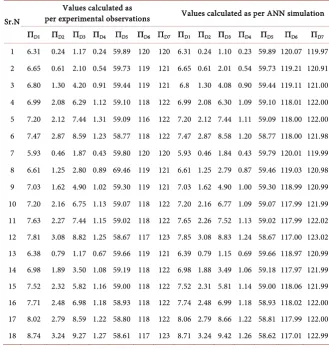
Table 1 shows the comparison of values calculated as per experimental

observa-tions and ANN simulaobserva-tions [5] [6]. The term such as πD1, πD2, πD3, πD4, πD5, πD6, πD7 indicates angles of Kingpin, Camber, Caster, Toe, Toe in, Toe out, Scrub

ra-dius respectively.

4. Procedure for Formulation of ANN Model

The experimental data based modeling has been achieved based on experimental data for the seven dependent pi terms. In such complex phenomenon involving non-linear kinematics where in the validation of experimental data based models

Table 1. Values computed by experimental observation and ANN simulation.

Sr.N

Values calculated as

per experimental observations Values calculated as per ANN simulation

ΠD1 ΠD2 ΠD3 ΠD4 ΠD5 ΠD6 ΠD7 ΠD1 ΠD2 ΠD3 ΠD4 ΠD5 ΠD6 ΠD7

(4)

is not in close proximity, it becomes necessary to formulate Artificial Neural Network (ANN) Simulation of the observed data. Simulation consists of three layers. First layer is known as input layer. The input neurons in input layer are equal to the number of independent variables. Second layer is known as hidden layer. It consists of seven numbers of neurons. The third layer is output layer. It contains one neuron as one of dependent variables at a time. For the ANN mul-tilayer feed forward topology is decided.

MATLAB software is selected for developing ANN simulation. The following steps are involved for developing the ANN algorithm is as under.

• _{The experimental data is separated into two parts viz. input data and the}

output data pi terms. The input data and output data are imported to the program respectively.

• _{The prestd function is used to read the input and output data and}

appro-priately sized.

• _{The input and output data is normalized in preprocessing step using mean}

and standard deviation.

• _{The input and output data is then categorized in three categories viz. testing,}

validation and training. From the 18 observations, initial 75% of the observa-tions is selected for training, last 75% data for validation and middle overlap-ping 50% data for testing.

• _{The data is then stored in structures for training, testing and validation.} • _{The feed forward back propagation is selected based on the data.}

• _{Using the training data the network is then trained. The actual data and}

tar-get data are compared and simulate the network.

The regression analysis and the representation are done through the standard functions. The values of regression coefficient and the equation of regression lines are represented on the seven different graphs plotted for the seven depen-dent pi terms [7] [8]. The detailed ANN program used for evaluation the steer-ing geometry is provided in the Appendix.

ANN Model

Figure 1 shows the structure and basic elements for designing artificial neural

(5)

[image:5.595.220.530.75.213.2]

DOI: 10.4236/eng.2019.114016 235 Engineering Figure 2. ANN neurons with its elements [3] [4].

Figure 3. ANN topology.

program shown in Appendix is run on the MATLAB software. The ANN

Out-puts consists of all the steering parameters are shown in the Table 1.

5. Conclusion

[image:5.595.220.529.114.522.2]

(6)

Conflicts of Interest

The author declares no conflicts of interest regarding the publication of this pa-per.

References

[1] Gillespie, T.D. (1992) Fundamentals of Vehicle Dynamics. Society of Automotive Engineers Inc., Warrendale.

[2] Suh and Redcliff (1978) Kinematics Design of Mechanisms. John Wiley and Sons, New York.

[3] Sivanandam, S.N., Sumathi, S. and Deepa, S.N. (2006) Introduction to Neural Net-works Using Matalb 6.0. Tata Mcgraw-Hill Publishing Company Limited, New Del-hi.

[4] Kartalopoulos, S.V. (2004) Understanding Neural Networks and Fuzzy Logic—Basic Concepts and Applications. Publication Prentice Hall of India Private Limited, New Delhi.

[5] Schenck Jr., H. (1961) Theory of Engineering Experimentation. Mc Graw Hill. [6] Belkhode, P.N. and Modak, J.P. (2011) Comparison of Steering Geometry

Parame-ter of Front Suspension of Automobile. Internal Journal of Scientific and Engineer-ing Research, 3, 1-3.

[7] Belkhode, P.N. and Modak, J.P. (2007) Kinematic Analysis of Front Suspension of an Automobile and Steering Behaviour. Proceedings of 12th World Congress in Mechanism and Machine Science, Besancon, 17-21 June 2007.

(7)

Appendix

ANN Program clear all;

close all; inputs3=[ ]

a1=inputs3 input_data=a1; output3=[ ]

y1=output3 size(a1); size(y1); p=a1'; sizep=size(p); t=y1'; sizet=size(t); [S Q]=size(t)

[pn,meanp,stdp,tn,meant,stdt] = prestd(p,t);

net = newff(minmax(pn),[18 1],{'logsig' 'purelin'},'trainlm'); net.performFcn='mse';

net.trainParam.goal=.01; net.trainParam.show=200; net.trainParam.epochs=50; net.trainParam.mc=0.05; net = train(net,pn,tn); an = sim(net,pn);

[a] = poststd(an,meant,stdt); error=t-a;

x1=1:18;

plot(x1,t,'rs-',x1,a,'b-')

legend('Experimental','Neural');

title('Output (Red) and Neural Network Prediction (Blue) Plot'); xlabel('Experiment No.');

ylabel('Output'); grid on;

figure

error_percentage=100*error./t plot(x1,error_percentage) legend('percentage error'); axis([0 18 -100 100]);

title('Percentage Error Plot in Neural Network Prediction'); xlabel('Experiment No.');

(8)

grid on; for ii=1:18

xx1=input_data(ii,1); yy2=input_data(ii,2); zz3=input_data(ii,3); xx4=input_data(ii,4); yy5=input_data(ii,5); zz6=input_data(ii,6); xx7=input_data(ii,7); pause

yyy(1,ii)

yy_practical(ii)=(y2(ii,1)); yy_eqn(ii)=(yyy(1,ii)) yy_neur(ii)=(a(1,ii))

yy_practical_abs(ii)=(y2(ii,1)); yy_eqn_abs(ii)=(yyy(1,ii)); yy_neur_abs(ii)=(a(1,ii)); pause

end figure;

plot(x1,yy_practical_abs,'r-',x1,yy_eqn_abs,'b-',x1,yy_neur_abs,'k-'); legend('Practical','Equation','Neural');

title('Comparision between practical data, equation based data and neural based data');

xlabel('Experimental'); figure;

plot(x1,yy_practical_abs,'r-',x1,yy_eqn_abs,'b-'); legend('Practical’,’ Equation');

xlabel('Experimental'); figure;

plot(x1,yy_practical_abs,'r-',x1,yy_neur_abs,'k-'); legend('Practical','Neural');

xlabel('Experimental');

error1=yy_practical_abs-yy_eqn_abs figure

error_percentage1=100*error1./yy_practical_abs; plot(x1,error_percentage,'k-',x1,error_percentage1,'b-'); legend('Neural','Equation');

axis([0 100 -100 100]);

(9)

Predic-DOI: 10.4236/eng.2019.114016 239 Engineering

tion');

xlabel('Experiment No.'); ylabel('Error in %'); meanexp=mean(output3) meanann=mean(a)

meanmath=mean(yy_eqn_abs)

mean_absolute_error_performance_function = mae(error) mean_squared_error_performance_function = mse(error)

net = newff(minmax(pn),[18 1],{'logsig' 'purelin'},'trainlm','learngdm','msereg'); an = sim(net,pn);

[a] = poststd(an,meant,stdt); error=t(1,[1:18])-a(1,[1:18]);

net.performParam.ratio = 20/(20+1); perf = msereg(error,net)

rand('seed',1.818490882E9) [ps] = minmax(p);

[ts] = minmax(t); numInputs = size(p,1); numHiddenNeurons = 18; numOutputs = size(t,1);

net = newff(minmax(p), [numHiddenNeurons,numOutputs]); [pn,meanp,stdp,tn,meant,stdt] = prestd(p,t);

[ptrans,transmit]=prepca(pn,0.001); [R Q]=size(ptrans);

testSamples= 6:1:Q; validateSamples=15:1:Q; trainSamples= 1:1:Q;

validation.P=ptrans(:,validateSamples) ; validation.T=tn(:,validateSamples) ; testing.P= ptrans(:,testSamples) ; testing.T= tn(:,testSamples) ptr= ptrans(:,trainSamples) ; ttr= tn(:,trainSamples);

net = newff(minmax(ptr),[18 1],{'logsig' 'purelin'},'trainlm'); [net,tr] = train(net,ptr,ttr,[] ,[],validation,testing);

plot(tr.epoch,tr.perf, 'r',tr.epoch,tr.vperf, 'g',tr.epoch,tr.tperf, 'h') ; legend('Training', 'validation', 'Testing',-1) ;

ylabel('Error') ; an=sim(net,ptrans); a=poststd(an,meant,stdt); pause;

figure