A New Algorithm of Mobile Node Localization
Based on RSSI
Jie Zhan1, Hongli Liu1, Bowei Huang2
1College of Electrical and Information Engineering, Hunan University, Changsha, China; 2College of Information and Electrical En-gineering, Hunan University of Science and Technology, Xiangtan, China.
Email: {JieZhanwl, kane.rex}@163.com, [email protected]
Received March 8th, 2011; revised March 22nd, 2011; accepted March 25th, 2011.
ABSTRACT
Position mobile node coordinate is a key component to determine the accuracy and efficiency of positioning in wireless sensor networks. Flexible location algorithm admits to adjust the accuracy and time cost of positioning based on the users references. This paper develops a location algorithm named Signal Strengthening Dynamic Value (SSDV) based on the database of RSSI to position the mobile node in terms of the value of beacon nodes RSSI. The proposed algo-rithm has successfully improved the accuracy of mobile nodes positioning and real-time, and simulation results show high performance in effectiveness of the algorithm.
Keywords: RSSI, Wireless Sensor Networks, Mobile Location Position, Signal Strength, Weight
1. Introduction
The algorithms of wireless sensor networks(WSN) posi-tion can be divided into two main categories [1]—
Range-based position and Range-free position. in the Range-based position algorithm, we need to measure the distance and angle between the mobile nodes and the beacon nodes, and then count out the position of the mo-bile nodes by Tri-lateral measurements, Triangular mea- surements or Maximum likelihood estimation method. Yet, in the Range-free position algorithm, we need only information of the network-connectivity and signal strength. Here, non-distance-position method has a great superiority owing to that it has no requirements for accu-rate distance-measuring so that the cost of the hardware establishments will be greatly reduced and thus can be large-scale installed, and the precision of the position can be improved by algorithm. At present, the Range-free method has been widely used in the convex program [2], the DV-Hop [3] and etc. However, the convex program method requires that the reference nodes located on the edge of the network, otherwise the position will deflect towards the center; while the DV-Hop algorithm can carry out accurate position only in intensive isotropy networks [4]. The so-called isotropy here means that the
signal strength will not change with the orientation of measures. However, it is hardly to guarantee the isotropy of the network in the indoor. Thus, the SSDV (Signal Strengthening Dynamic Value) scheme discussed in this article is born out of an algorithm of positioning which uses the Range-free techniques, and can accurately per-ceive the movements of the measuring objects. Thus it is very suitable to be used indoor. In our discussing, we assume that the wireless-signals can be kept steady and the signal covering scale of the nodes is a standard round area.
2. Principle of Distance Measurements of
RSSI
An important feather of wireless signal transmission is that the signal strength decreases as the distance increase. The principle of distance measurements of RSSI is to change attenuation of the signal strength into distance of signal transmission, using the functional relation between attenuation of the signal and the distance approximately. Researchers have done some effective researches about signals in different transmission environment [5], and conclude some good empirical formula:
1 10 log
d
L L dv (1)
Foundation Item:Hunan Provincial Science and Technology Plan Pro-ject (No.2010FJ4068); National Laboratory for Infrared Physics, Chi-nese Academy of Sciences (201021).
2
1 10 log t r 4π
c f L G G
t is Transmitting antenna gain, r is Receiver
an-tenna gain, c is velocity of light, f is carrier frequency,
G G
Channel attenuation coefficient (2~6), v is the Gaus-sian random variable which considered the shadow effect, then v~N
0, 2is
, d is the distance, Ld is the channel
loss after the distance d.
In practice, we get the relation between RSSI and the distance through the measurement of transmission power and receiving power. Most of the chips which provide RSSI measurement show the relation of transmission power and receiving power by the following formula:[6]
n R T
P P r (3)
After the conversion was:
10 lgR
P dBm A n r (4)
R
P is the receiving power of the wireless signal, T
is transmission power, n is the Propagation factor, r is the distance between Transceiver Unit. A is the receiving signal power when the signal transmit 1 meter. The nu-merical value of constant A and n determined the relation between receiving signal strength and signal transmission distance.
P
As to different chips, the empirical formula has corre-sponding different form due to different hardwire and modulation. The chip CC2430 used in our experiment is based on the IEEE802.15.4 agreement, using the DSSS,
O-QPSK modulation technology in the physical layer. IEEE802. 15. 4 gives the simplified channel model [7]
40.2 10 2 lg58.5 10 3.3 lg 8 m8 mt t
RSSI d P d d
RSSI d P d d
(5)
Most of theoretical analysis and empirical formula show that the relationship between RSSI and the trans-mission distance of wireless signal is apparent. The measurement of RSSI has repeatability and interchange ability, and there is a pattern in the application environ-ment when RSSI does appropriate changes. After having finished the environmental factors, RSSI can do the dis-tance measurement of indoor and outdoor.
3. Ranging Experiment and Processing
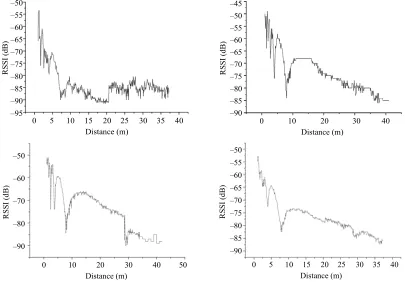
In order to do a comprehensive discussion of RSSI rang-ing, we designed the following experiment. Do four groups ranging experiment which is mutually perpendicularity on an empty space, the nodes are above the ground one meter. The mobile node and fixed node start the ranging from the position one meter away, every 0.1 meter as a measuring point, and every measuring point will be measured 10 times. After 42 meters measured, part of the signals is not detected, because the RSSI values is ob-tained from complete receiving data packets, so the test is meaningless to continue. The four groups of experi-mental results are shown in the Figure 1.
Distance (m)
0 5 10 15 20 25 30 35 40
RSSI
(
dB)
–50 –55 –60 –65 –70 –75 –80 –85 –90 –95
Distance (m)
0 10 20 30 40
RSS
I (d
B)
–50 –55 –60 –65 –70 –75 –80 –85 –90 –45
Distance (m)
0 10 20 30 40 50
RSS
I (
dB)
–50
–60
–70
–80
–90
Distance (m)
0 5 10 15 20 25 30 35 40
R
SSI (d
B
)
[image:2.595.96.501.424.706.2]–50 –55 –60 –65 –70 –75 –80 –85 –90
We have collected 16000 experimental data, and the analysis on those statistics shows that: Each RSSI value corresponds to an distance scope, and high-intensity val-ues has small probability, low-intensity valval-ues has large probability. So we can find the highest density peaks and filter out most wrong dates by doing Gaussian fitting. The probability distribution Restructure is shown in the
Figure 2. There is only one peak for each different RSSI
measurement value, and the peak is steeper as the value is bigger, then the error is small, the peak is more slowly as the value is smaller, then the error become big. We get the fitting function:
2 2 ( ) 2
0 e
π 2
c
x x
A
y y
(6)
21 , 1
1
k k
i i
i i
c
RSSI RSSI x
x w
k k
c
It is hard to find out the RSSI peak value of each measurement point. The value can be substituted into (6), when 0.5 ≤ y ≤ 1,we consider it is a large probability event and can be reserved, then we obtain the determined RSSI value by taking the average of the reserved RSSI values. 0 and A are undetermined coefficients(can be determined by the relation between beacon nodes’ loca-tion and RSSI), k is the number of received beacon nodes.
y
Gaussian fitting reduced the influence of some low probability and large disturbance events by using Gaus-sian fitting to do data processing, and reduced the rang-ing error. Figure 3 is the data processing results
[image:3.595.309.533.544.710.2]com-pared to Gaussian fitting and mean approach. The result shows that Gaussian fitting is better than mean model in improving ranging precise, especially when we measure close distance, and the error can be control within 1.2 meters on open space.
Figure 2. Probability distribution of RSSI by Gaussian
fit-Figure 3. The distribution error of Gaussian fitting vs.
av-reference erage.
4. The Signal Strengthen Dynamic Value
Scheme (SSDV)
4.1. The Principle of Position
First, the SSDV builds up the data-base of the
nodes via the exchange nodes which keep on sending out signals, signals are received by the reference nodes and then the reference nodes send back information of the strength of the signals. Shown as Figure 4, the exchange
[image:3.595.61.284.555.695.2]nodes keep broadcasting signals which carry information of its ID and all the reference nodes and exchange nodes receive the signals and send back information of the sig-nals which it received and information of its own ID. With the data-base of the reference nodes, the positioning scheme can work even without reference nodes. When a mobile node needs to be positioned, it will send informa-tion of the signal strength of all the exchange nodes that it can receive together with a position requirement. The position procedure is as follows:
al
Suppose the mobile node as X, and B
b1, , bn
asetected by X,
1 n
l the exchange nodes that can be d the strength of the signals that X receives as
, ,
,
, ,
D d d as all the reference nodes
-As to every random dxD, the signal
strength of the exchange nodes received are supposed as
1 n
tioning region.
in the posi
1, , , , , x
b d b d
, du, dv are the two adjacent
v D
x n
u
d D,
reference nodes; d , HD
hd1, , hdn
is supposed as the focus ference odes; let re n HDDpositio
1 n
formed by 4 ,
, ,
S s s is supposed as the assistant
-onnects duand dv, and the value is
ex-pressed as Ws
ws , , w
; and C
c, , c
isthe minimum which is
ref-erence nodes in the positioning region. Here, we consider them as clusters. Let
1 n
ing-line that c
n
1
rectangle region s2
,
i i i
c D S , DiD, SiS ,
then HC
hc1, , hcn
s ; letstands for the focu clusters
HCC, then HC
h1, ,
o key c hc n
w w
.
S d out t node
W
he tw
tep 1: Fin exchange s. Suppose that uopt ui, uopt u1,un when i1,n, then
the e node obile
nodes; if the uwst ui, opt
b is the kernel exchang for the m
1 wst n
u u u when i1,n, the bwst is the s e e;
St : Find out all the focus nodes in terminu xchange nod
re
d
(7)
consider the assistant positioning-line that connects the
ep 2 the positioning
gion. When bopt can assure that
max , , ,
min , , ,
opt u opt v
opt opt u opt v
u b d u b d u u b d u b
couple of du, dv as sx, then all the cx sx are
fo-cus clusters nd hen we judge all the v in the
positioning region using Formula (2), we w g the HD and HC of the positioning region;
Step 3: Test whether X is positi
a w du, d
ill et
oned in the region. As for every randomly couple du , dv , let duHD ,
v
d HD, the following formula :
is
max , , ,
min , , ,
opt u opt v
opt opt u opt v
b d b d b d b d
(8)then it means that X is positioned in the region and the
atching step. If there exists positioning can go on; if there are no couples of du, dv,
u
d HD, dvHD accord with the Formula ), it
ositioned in the region and thus end the positioning procedure.
Step 4: Carry on the m
(8 means that X is not p
b d,
u , hdxHD, where the is athresh-lance the err brought by interference, then the position of
i x i
u
old value which is used to ba ors
x
hd is the position of
the mobile node and the position is ended. Otherwise, the position goes on.
Step 5: Calculate the value of the focus clusters. As for all du, dv, duHD, dvHD, and i1,n, let
the follow g fin ormula:
, ,
min , , ,
i u i v
i i u i
b d
b d b d
v
(9)come into existence for k times, then the value of the max b d,
assistant positioning-line which connects the couple of
u
d , dv expressed as wsx is k. All the values of
H to be calculate y Formula (9). Then, all S C d b
HC
W
St
can be calculated by formula: whc
S hc ws. ep 6: Carry on the matching step of clusters. If ere th exists an exclusive whcx whci, i1,n, then thecen-ter of this maximum of the mobile node and the position ends up; if whcx whcy whci,
1,
i n
cluster is the position
, at meantime, whcx and t
hen the center of cluster e up by these two clusters is the position of the mobile node and the position ends up.
4.2. The Charac
hcy
w
mad
are adjacen
clusters, t the
teristic of the Algorithm
[image:4.595.309.533.529.698.2]
circum-no
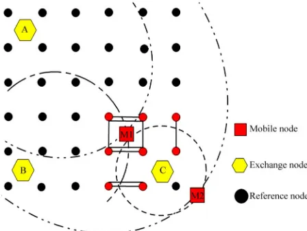
Figure 5 is the sketch map of the position. In
stances as shown in the figure, A, B, C stand for ex-change nodes and C is the nuclear exex-change node, A is the terminus exchange node; let M1, M2 be mobile nodes to be positioned, the small dots stand for reference nodes among which the brightened ones stand for hot clusters.
1) No blind spot in the positioning region. After the de-matching and the cluster-matching steps, the blind spots can be completely cleared up and this makes the originally unhandy Mass-Center Position Scheme much more flexible in that the positioning spot is not limited to only the mass center of the cluster but also the midpoint of the assistant positioning-line and places of reference nodes. Thus, the accuracy of the positioning will in-creased greatly.
2 r-m
her the mobile node is po
is a square plane with an ) Good real-time effect of positioning. Via the dete ining of hot cluster, the quantity of unnecessary calcu-lations will be greatly cut. As shown in Figure 1, when
positioning M1, it needs only to calculate the value of the cluster in the right-foot of the whole positioning region but no needs for any other ones.
3) Be able to determine whet
sitioned in the region. Via comparing the value of the assistant positioning–line produced by the terminus ex-change nodes with the value of the assistant position-ing-line produced by the nuclear exchange node, it is able to determine whether the mobile node is positioned in the positioning region. As shown in Figure 3, when
positioning M2, although the nuclear exchange node C can still produce a hot cluster in region shown in the fig-ure, however, as the terminus exchange node A does not bring out any value in the focus cluster, we can still de-termine that M2 is not positioned in the region.
5. Simulation Analysis
Suppose the positioning region
area of 50 × 50 m2, and on it an square region with an area of 40 × 40 m2 is distributed equably with reference
region and the space between the reference nodes is 5 m. the exchange nodes are positioned in the four point an-gles A, B, C, D of the positioning region.
The simulation result is shown in Figure 6. The black
line is the assistant positioning-line, the larger the value, the wider the line. The assistant with no value will not be shown. And the triangular shapes refer the focus refer-ence nodes region while the small square shapes refer the actual spot of the mobile nodes, and the stars are the places that are determined by calculation. In Figure 6(a),
the mobile node is positioned at coordinate (41, 39). The positioning result which is calculated by node-matching is coordinate (40, 40) with an error of 1.4142 m and time- cost of 28 ms. In Figure 6(b), the mobile node is
posi-tioned at coordinate (26, 28), and the calculated position-ing result is coordinate (25, 27.5) with an error of 1.118 m and time-cost of 43 ms. In Figure 6(c), the mobile node
is positioned at coordinate (13, 17), and the calculated positioning result is coordinate(12.5, 17.5) with an error of 0.7071 m and time-cost of 41 ms. In Figure 6(d), the
[image:5.595.98.498.378.709.2]mobile node is positioned at coordinate (48, 24), and the calculated positioning result shows that it does not exist in the positioning region with a time-cost of 29 ms.
From Figures 6(a) and (b), we ca
ca
s a new algorithm of SSDV. This
al-[1] F. B. Wang, “Self-Localization
rithms for Wireless Sensor Networks,” n see that the SSDV Systems and Algo
n determine the mobile nodes on special positions ac-curately; As from Figure 6(c), it shows that most mobile
nodes on normal positions can be determined accurately by this algorithm. From Figure 6(d), we can see that
when the mobile node is located out of the positioning region, the SSDV can find this out correctly. While comparing (a), (d) with (b), (c), we can see that the less the steps of the positioning, the less of the time-cost; while comparing (b) with (c), we can see that the closer is the mobile node near to any random reference node, the smaller the focus positioning region will be while the time cost is cut only with a very small quantity. On the contrary, the focus positioning region will get larger and the time-cost increase also has a very little quantity.
6. Conclusions
This paper present
gorithm needs only the strength of the radio signals as foundation to position the mobile nodes. The establish-ment is rather simple and there is no blind spot in tioning region, and the accuracy and the time of posi-tioning can both be adjusted by the users. The result of simulation proves the validity of this algorithm.
REFERENCES
L. Shi and F. Y. Ren,
Journal of Software, Vol. 16, No. 5, 2005, pp. 857-868. doi:10.1360/jos160857
[2] L Doherty, K. S. J. Pister and L. E. Ghaoui, “Convex Position Estimation in Wireless Sensor Networks,” Pro-ceedings of the 20th Annual Joint Conference of the IEEE Computer and Communications Societies, Anchorage, Vol. 3, 22-26 April 2001, pp. 1655-1663.
doi:10.1023/A:1023403323460
[3] D. Niculescu and B. Nath, “DV Based Positioning in Ad
iao and H.-C. Liao,
rod and D. Estrin, “Robust Range Estimation Using
Bychovskiy, J. Elson and D. Estrin, “Locat-Hoc Networks,” Journal of Telecommunication Systems, Vol. 22, No. 4, 2003, pp. 267-280.
[4] M.-H. Jin, E. H.-K. Wu, Y.-B. L
“802.11-Based Positioning System for Context Aware Applications,” Proceedings of Global Telecommunica-tions Conference, Vol. 2, 1-5 December 2003, pp. 929- 933.
[5] L. Gi
Acoustic and Multimodal Sensing,” Proceedings of the IEEE/RSJ International Conference on Intelligent Robots and Systems, Maui, 29 October-3 November 2001, pp. 1312-1320.
[6] L. Girod, V.
ing Tiny Sensors in Time and Space: A Case Study,” In: B. Werner, Ed., Proceedings of the IEEE International Conferenceon Computer Design: VLSI in Computers and Processors, Freiburg, 16-18 September 2002, pp. 214-219. [7] J. Zhan, L.-X. Wu and Z.-J. Tang, “Research on Ranging