Study on Productivity Model of Herringbone Like Laterals Wells and Optimization of Morphological Parameters Considering Threshold Pressure Gradient in Heavy Oil Reservoirs

http://www.scirp.org/journal/wjet ISSN Online: 2331-4249 ISSN Print: 2331-4222

DOI: 10.4236/wjet.2019.72021 May 8, 2019 302 World Journal of Engineering and Technology

Study on Productivity Model of

Herringbone-Like Laterals Wells and

Optimization of Morphological Parameters

Considering Threshold Pressure Gradient in

Heavy Oil Reservoirs

Enhui Sun

, Jie Tan, Dong Zhang, Wei Wang, Songru Mu

Bohai Oilfield Research Institute of CNOOC Ltd.-Tianjin Branch, Tianjin, China

Abstract

Compared with conventional well, herringbone-like laterals wells can in-crease the area of oil release, and can reduce the number of wellhead slots of platforms, and also can greatly improve the development efficiency. Based on threshold pressure gradient in heavy oil reservoir, and the applied principle of mirror reflection and superposition, the pressure distribution equation of herringbone-like laterals wells is obtained in heavy oil reservoir. Productivity model of herringbone-like laterals wells is proposed by reservoir-wellbore steady seepage. The example shows that the productivity model is great accu-racy to predict the productivity of herringbone-like laterals wells. The model is used to analyze the branching length, branching angle, branching symme-try, branching position and spacing and their effects on productivity of ringbone-like laterals wells. The principle of optimizing the well shape of her-ringbone-like laterals wells is proposed.

Keywords

Threshold Pressure Gradient, Herringbone-Like Laterals Wells, Heavy Oil Reservoirs, Productivity Model, Optimization of Morphological Parameters

1. Introduction

Compared with the onshore oilfields, the number of wellhead slots is limited in offshore oilfields. The herringbone-like laterals wells not only increase the drai-nage area and single well-controlled reserves, but also increase the production of How to cite this paper: Sun, E.H., Tan, J.,

Zhang, D., Wang, W. and Mu, S.R. (2019) Study on Productivity Model of Herring-bone-Like Laterals Wells and Optimization of Morphological Parameters Considering Threshold Pressure Gradient in Heavy Oil Reservoirs. World Journal of Engineering and Technology, 7, 302-313.

https://doi.org/10.4236/wjet.2019.72021

Received: April 1, 2019 Accepted: May 5, 2019 Published: May 8, 2019

Copyright © 2019 by author(s) and Scientific Research Publishing Inc. This work is licensed under the Creative Commons Attribution International License (CC BY 4.0).

http://creativecommons.org/licenses/by/4.0/

DOI: 10.4236/wjet.2019.72021 303 World Journal of Engineering and Technology

oil wells; it has certain advantages in offshore oilfield development. Therefore, it is necessary to study the productivity prediction of herringbone-like laterals wells in reservoirs. In 1996, Salas [1] assumed each branch is divided into several segments and established analytical model of single-phase seepage in fishbone multi-branch horizontal wells. In 2004, Han Guoqin [2] and He Haifeng [3] es-tablished a steady seepage mathematical model of fishbone multi-branch wells considering the flow in the wellbore. Liu Xiangping, Yang Xiaosong, Zhao Guang, et al. [4] [5] [6] [7] [8] deduced the productivity calculation model of fishbone horizontal well by potential superposition principle. Based on the prin-ciple of equivalent seepage resistance and productivity formula of horizontal wells, a simple productivity formula for fishbone horizontal wells is derived by Li Chunlan [9]. Fan Yuping, Ye Shuangjiang, Zhang Shiming, et al. [10] [11] [12]

used numerical simulation method to study the productivity of herringbone-like laterals wells. Because heavy oil is affected by threshold pressure gradient, the above research is not suitable for predicting the productivity of wells in heavy oil reservoirs. Considering the influence of threshold pressure gradient on heavy oil reservoir, herringbone-like laterals wells coupling productivity model for reser-voir-wellbore steady seepage is proposed; the example shows that the productiv-ity model is high accuracy in predicting the productivproductiv-ity of herringbone-like erals wells, and the principle of well shape optimization for herringbone-like lat-erals wells is proposed.

2. Pressure Distribution Considering Threshold Pressure

Gradient

In reference [13], porous media conditions, heavy oil reservoir seepage law is non-Darcy seepage with threshold pressure gradient. When the driving pressure gradient exceeds its initial pressure gradient, heavy oil begins to flow and its seepage characteristics are shown in Figure 1. Among them, A is the minimum threshold pressure gradient, B is the average threshold pressure gradient; C is the maximum threshold pressure gradient.

The law of non-Darcy seepage can be described by the following formula:

DOI: 10.4236/wjet.2019.72021 304 World Journal of Engineering and Technology

d d

,

d d

K p p

v

r λ r λ

µ

 

= − _ − _ >

  (1)

where v is seepage velocity, m3_{/s; K is reservoir permeability, mD;} d d p

r is

pres-sure gradient, MPa/m; λ is threshold pressure gradient, MPa/m. when K p

µ

Φ = _{, have:}

d d K K v r λ µ µ Φ

= − + (2)

Assuming that the formation is infinitely homogeneous and isotropic, there is a horizontal well in which the length of the horizontal well is L, the coordinates of the two ends of the well are (x1, 0, zw), (x1, 0, zw), setting the horizontal well is homogeneous line sink, the productivity of the well is Q, the productivity of per unit length L is q, selecting micro-element dx0 at x0 of horizontal well. It can be regarded as the seepage velocity of M(x0, y0, z0) at any point:

2

4π q v

r

= ₍₃₎

A new velocity potential function considering threshold pressure gradient at point M is obtained:

(

) (

) (

)

0

2 2 2

0 0 0

d d d 4π D x Q K R C

L _{x x y y z z} λµ

Φ = − + +

− + − + − (4)

where RD is the shortest distance between the micro-element and the moving

boundary.

According to the superposition principle of potential, the velocity potential caused by the whole horizontal well is as follows:

(

) (

) (

)

2

1

0

2 2 2

0 0 0

d 4π x D x x Q K R c

L _{x x y y z z} λ µ

Φ = − + +

− + − + −

∫

In this paper, a horizontal well is divided into N segments by mathematical discretization method. As the productivity of the well varies little in a small sec-tion, it can be assumed that the productivity of this section is a fixed value, and the production of each section is different:

(

) (

) (

)

1

1

0

2 2 2

0

0 0 0

d 4π i i x N D

i i x

x

Q K

R c

L _{x x y y z z} λ µ

+

−

=

 

  _′

Φ = _− _+ +

 _{− + − + −} 

 

∑

∫

As the horizontal well is parallel to the X-axis and on the XOY plane, so

0

y =y, z0 =zw, the Formula (6) is changed to:

( )

(

₍

)

₎

1 1 0 ln 4π N i i D

i i i i

x x r

Q K

M R c

L x x r λ µ

−

+ +

=

− +

′

Φ = − + +

− +

∑

where

(

)

(

)

i i w

r = x −x +y + z −z .

branch-DOI: 10.4236/wjet.2019.72021 305 World Journal of Engineering and Technology

ing). The herringbone-like laterals wells are divided into several segments. And it is setted the flow rate of section s of the branching t. According to the super-position principle of mirror reflection and potential, potential produced by her-ringbone-like laterals wells system at any point M in reservoir:

( )

(

(

[ ][ ] [ ][ ]

)

(

[ ][

] [ ][

]

)

)

[ ][ ] [ ][ ]

(

)

(

[ ][

] [ ][

]

)

(

)

[ ][ ] [ ][ ]

(

)

(

[ ][

] [ ][

]

)

(

)

[ ][ ] [ ][ ]

(

)

(

[ ][

] [ ][

]

)

(

)

(

)

, , 4 , 1 , 1 , 4 ,

, , 4 2 , 1 , 1 , 4 2 ,

, , 4 , 1 , 1 , 4 ,

, , 4 2 , 1 , 1 , 4 2 ,

M N

ts w w t

k t s

w w t

w w t

w w t

e

M x t s y t s kh z x t s y t s kh z

x t s y t s kh h z x t s y t s kh h z

x t s y t s kh z x t s y t s kh z

x t s y t s kh h z x t s y t s kh h z

K R x ϕ α ϕ α ϕ α ϕ α λ µ +∞ − =−∞ = = 

Φ = _ + + + +

+ + − + + + − − − + + −  − − + + + − + _ + −

∑ ∑ ∑

[ ][ ] [ ][ ]

(

)

(

[ ][

] [ ][

]

)

(

)

, , 4 2 , 1 , 1 , 4 2 ,

ln 4π

w w t

ts ts ts ts

ts

ts ts ts ts

x t s y t s kh h z x t s y t s kh h z

q r r L

c

L r r L

ϕ α + + + − + + + − + + = − + + −

(

) (

) (

)

4 2

ts ts ts w

r = x −x + y −y + kh+ h−z −z , m; L_ts is the length of the

s segment of the branching t, m; k is infinite well row reflected by mirror image of branching in Z direction.

The wellbore pressure distribution equation of herringbone-like laterals wells wells under bottom water reservoir is obtained according to Equation (8):

(

)

wts e ets ts

p p

K µ

= + Φ − Φ ₍₉₎

For bottom water reservoirs, there is: 0

ets

Φ = ₍₁₀₎ The FORMULA (9) is changed to:

wts e ts

p p

k

µ

= − Φ ₍₁₁₎

where µ is oil viscosity, mPa·s; K is reservoir permeability, mD; pwts is the

well bottom hole flow pressure of the s segment of the branching t, MPa; pe is

initial reservoir pressure, MPa.

3. Pressure Drop Equation of Wellbore Flow

3.1. Computational Model of Flow Pressure Drop in Main and

Branch Wellbore

The main wellbore and branching wellbore are divided into many units. Consi-dering that the length of each unit is enough small, the pressure drop of the second section of the branching t of herringbone-like laterals wells is calculated in reference [14]:

(

)

(

)

2 5 2 4

2 16

2 2

π π

hw ts

wts ts ts ts ts

f q

p Q q x Q q

D D

ρ

ρ

DOI: 10.4236/wjet.2019.72021 306 World Journal of Engineering and Technology

where qts is radial inflow of micro-element section in the s segment of the

branching t, m3_/s;

ts

Q is the upstream flow of the mainstream for the s segment

of branching t, m3_/s;

hw

f is friction resistance coefficient of the well tube wall

with radial inflow, f; ρ is fluid density, kg/m3_{; D is the wellbore diameter, m.}

3.2. Computational Model of Convergent Flow Pressure Drop of

Main and Branching Wellbore

While the fluid of the main wellbore and branching wellbore is confluencing, a mixed loss will occur, and generated local pressure drop. Based on the principle of fluid mechanics, a calculation model of local pressure drop at the confluence point of main wellbore and branching wellbore is established.

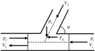
Assuming that the fluid in the wellbore flows steadily, adiabatically and iso-thermally, without considering the friction between the fluid and the pipe wall, and ignoring the influence of gravity, the confluence flow diagram of the branching wellbore is shown in Figure 2.

The momentum equation of the main wellbore direction of the fluid at the confluence point is as follows:

2 2

1 2 2 2 1 1

π π

4 4 x

p D −p D +F =ρQ V −ρQ V (13)

Continuity equation:

2 2

1 2

π π

4 t 4

V D +q =V D (14)

Energy equation:

2 2

1 1 2 2

12

2 2

p V p V

h

g g g g

ρ + = ρ + + (15) where p1, p2 are pressure at the inflow and outflow ends along the direction

of the main wellbore at the confluence point, MPa; D is main wellbore and branching wellbore diameter, m; qt is from the branching wellbore t to main

wellbore, m3_/s.

The force Fx of the wall acting on the gas at the junction point can be

de-rived from the momentum equation:

3cos

x t

F =ρq V ϕ (16)

Combination the Formula (13) and (16):

(

)

1 2 2 2 2 1 1 3

4

cos

π t

p p Q V Q V q V

D

ρ

_ϕ

− = − − (17)

Combination the Formula (14), (15) and (17), pressure drop equation at the confluence point of main and branching wellbore is:

2

1 3 1 2 2 4 2 2

16 8 4

cos

π π π

t t t

wt

q V q V q

p p p

D D D

ρ ρ ρ _ϕ

∆ = − = + − (18)

Substitute 1 2

4 π

t

Q V

D

= , 3 2

4 π

t

q V

D

DOI: 10.4236/wjet.2019.72021 307 World Journal of Engineering and Technology Figure 2. Confluence flow diagram of main and branch wellbore.

(

)

2

1 2 2 4 2 4

16 32

1 cos

π π

t t t

wt

q Q q

p p p

D D

ρ _ϕ ρ

∆ = − = − + (19)

where Qt is flow from upstream end of the point of main wellbore t, m3/s; qt

is flow from branching wellbore t to the main wellbore, m3_{/s; ϕ is the angle of} branching, degrees; D is diameter of the main wellbore and branching wellbore, m.

4. Coupling Model of Seepage and Wellbore Flow in

Herringbone-Like Laterals Wells

In addition to flowing along the length of horizontal wellbore, reservoir fluid al-so flows into wellbore along the horizontal wellbore direction. There is a coupl-ing relationship between seepage flow in reservoir and in the wellbore.

4.1. Establishment of Coupling Model

The pressure distribution in wellbore can be calculated by the pressure drop calculation model as:

( )1 0.5

(

)

(

)

wts wt s wt s wts

p = p ₋ + ∆p ₋ + ∆p ≤ ≤t M− ≤ ≤s N (20)

0 0

wt

p

∆ = _, p_wt0= p_wft

where pwft is the flow pressure at the heel of the branching wellbore t, MPa; wts

p is the flow pressure of s segment of the branching t, MPa; p_{wt s(−1)} is the flow pressure of s−1 _{segment of the branching t, MPa;}

( )1 wt s

p ₋

∆ is the pressure drop of s−1 _{segment of the t branch, MPa;}

wts

p

∆ _{is the pressure drop of s} seg-ment of the branching t, MPa.

According to the principle of material balance, the inflow of each branching wellbore equals the sum of the inflow of each small section at the upstream:

1

0 =1

M N

ts ts

t s

Q q

−

=

=

∑ ∑

As can be seen from the above, the reservoir seepage model has m n×

equa-tion, the wellbore pressure drop model has m n× equation, there are 2m n× equations. The variables to be solved are qts and pwts

(

)

4.2. Solution of Coupled Model

fol-DOI: 10.4236/wjet.2019.72021 308 World Journal of Engineering and Technology

lows: 1) Assuming that the initial value of pwts is

0 wts

p , in actual calculation it can be assumed 0

wts wft

p = p ; 2) Substitute p_wts into the Formula (11), used

gauss elimination method to find qts; 3) Substitute qts into the Formula (21),

find Qts; 4) Substitute qts and Qts into the Formula (12) and (19), find wts

p

∆ _{; 5) Substitute} ∆pwts into the Formula (20), to update pwts. This value is

taken as the initial value of the next iteration; 6) repeat (2) - (5), comparing 1

n wts

p+ , q_tsn+1 after n iterations with pn_wts and q_tsn after n iterations, when both of them satisfied certain accuracy, the iteration stops, otherwise repeat (2) - (5) steps until the accuracy is satisfied; 7) Last, the Formula (21) can be used to cal-culate the total production of herringbone-like laterals wells.

5. Case Study and Optimization of Morphological

Parameters

5.1. Example Analysis

The herringbone-like laterals wells in a heavy oil reservoir in Bohai Oilfield as an example, the well pattern is shown in Figure 3. There are four branching along the main wellbore. The distance between each branching is 50 m, the angle be-tween the main wellbore and the branching wellbore is 45 degrees, the length of the main wellbore is 400 m, the length of each branching wellbore is 200 m, and the radius of the main wellbore and the branching wellbore is 0.119 m, reservoir thickness h=6.9 m, distance from the well to bottom of reservoir Zw=3.45 m, reservoir permeability 3 2

3159 10 m

K= × − µ , initial reservoir pressure 11.47 MPa

e

p = , bottom hole flow pressure pw =10.47 MPa , production pressure drop ∆ =p 1 MPa , branching wellbore radius rw =0.119 m , wall roughness e=0.001 m, oil viscosity µ=50 mPa s⋅ , volume coefficient of oil

1.07

B= , oil density ρ=0.969 g cm3, the threshold pressure gradient of the

reservoir is 0.02 MPa−1_/m.

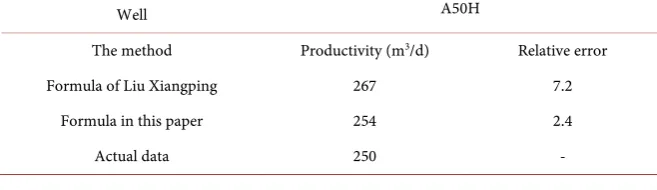
The productivity coupling model deduced by the author is used to predict the productivity of herringbone-like laterals wells. Compared with the actual pro-duction data, as shown in Table 1, it can be seen from Table 1 that the relative error between the calculated results and the actual production is less than that calculated by Liu Xiangping formula, which is 7.2%. The main reason is that the effect of threshold pressure gradient on productivity is considered in this paper. This formula has high practicability for predict the productivity of herring-bone-like laterals wells.

Table 1. Comparison of actual data and productivity of herringbone-like laterals wells.

Well A50H

The method Productivity (m3_{/d) Relative error}

Formula of Liu Xiangping 267 7.2 Formula in this paper 254 2.4

DOI: 10.4236/wjet.2019.72021 309 World Journal of Engineering and Technology Figure 3. Well pattern of herringbone-like laterals wells.

5.2. Study on Optimization of Morphological Parameters

The reservoir-wellbore steady seepage coupling model is used to optimize the shape of herringbone-like laterals wells, for give full play to the advantages of herringbone-like laterals wells.

1) Branching length optimization

The optimization of branching length mainly studies during the total wellbore length is equal, the productivity difference between equal and unequal branching length. In the study, the structure of two branching shown in Figure 4. The total length of the main wellbore and branching wellbore is 800 m, and the angle of each branching is 45 degrees.

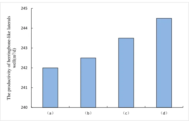
Figure 5 shows that when the total length of the wellbore is equal, during the length of the main wellbore and branching wellbore is increased; the productivi-ty of the well is increased. When the branching length is 0 m, the well will be transformed into a single horizontal well, that is, the productivity of a single ho-rizontal well is greater than an equal length herringbone-like laterals wells.

2) Branching angle optimization

Using the three branching structures as an example, the effect of branching angle on productivity is studied. As can be seen from Figure 6, the total angle of the three branching structures is 135 degrees. The productivity variation law is studied by changing the angle of each branching. The main wellbore and branching wellbore length are 400 m and 200 m respectively.

From Figure 7, it can be seen that the productivity of the well is the smallest when the branching angle is equal and the productivity is increased with the in-crease of the angle difference. Generally, the change of branching angle has little effect on the total productivity of the well, less than the influence of branching length.

3) Branching symmetry optimization

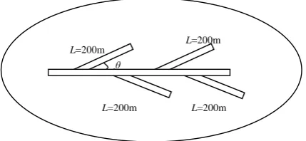
In order to study the effect of branching symmetry on productivity of the well, four branching structures are designed as shown in Figure 8. This paper mainly analyses whether there are common convergence points between the branching and the influence of the branching on the productivity of the well. The main wellbore length is 400 m, the branching wellbore length is 200 m, and the angle of each branching is 45 degrees.

As can be seen from Figure 9, that the ipsilateral branching structure will

L=200m

L=200m

L=200m

L=200m

DOI: 10.4236/wjet.2019.72021 310 World Journal of Engineering and Technology

contribution more productivity than opposite side branching structure. During the number of branching on one side of the main wellbore is increasing, the in-terference on the one side of the main wellbore is increasing, and the driving area of each branching is increasing. The result of comprehensive action in-creases the total productivity of the well.

4) Branching location and spacing optimization

In order to study the influence of branching location and spacing on the productivity of the well, four branching structures are designed as shown in

Figure 10. The main wellbore length is 400 m, the branching wellbore length is 200 m, the angle of branching is 45 degrees, and the distance between the main wellbore and the branching heel is shown in Figure 10.

As can be seen from Figure 11, that during the branching is closer to the heel of the main wellbore, the productivity of the well is larger. When branching spacing is increased the interference of branching is decreased, but the interfe-rence range of main wellbore is increased, the result of comprehensive action decreases the total productivity of the well.

Figure 4. Schematic diagrams of herringbone-like laterals wells with different branching length.

Figure 5. The productivity of herringbone-like laterals wells with different branching length.

(a)

② ①

(d) (c)

(b)

② ①

② ①

② ①

200m 200m

100m

100m

300m

300m

100m

239 240 241 242 243 244 245

（a） （b） （c） （d）

T

he

p

ro

d

uc

ti

vi

ty

o

f

he

rr

ingb

o

ne

-lik

e la

te

ra

ls

w

ell(

m

3/d

DOI: 10.4236/wjet.2019.72021 311 World Journal of Engineering and Technology Figure 6. Schematic diagrams of herringbone-like laterals wells with different branching angle.

Figure 7. The productivity of herringbone-like laterals wells with different branching angle.

Figure 8. Schematic diagrams of herringbone-like laterals wells with different branching symmetry.

240 241 242 243 244 245

（a） （b） （c） （d）

T

he

p

ro

d

uc

ti

vi

ty

o

f

he

rr

ingb

o

ne

-lik

e la

te

ra

ls

w

ell(

m

3/d

)

(a) (b)

(c)

② ④

③ ①

② ③ ④

① ②

④ ③

①

(d)

② ④

DOI: 10.4236/wjet.2019.72021 312 World Journal of Engineering and Technology Figure 9. The productivity of herringbone-like laterals wells with different branching symmetry.

Figure 10. Schematic diagrams of herringbone-like laterals wells with different branching location and spacing.

Figure 11. The productivity of herringbone-like laterals wells with different branching branching location and spacing.

236 237 238 239 240 241 242 243

（a） （b） （c） （d）

T

he

p

ro

d

uc

ti

vi

ty

o

f

he

rr

ingb

o

ne

-lik

e la

te

ra

ls

w

ell(

m

3/d

)

(a)

(d) (c)

(b) 350m

50m

② ①

50m

②

150m

①

②

250m 150m

① ① ②

350m 250m

246 247 248 249 250 251 252 253

（a） （b） （c） （d）

T

he

p

ro

d

uc

ti

vi

ty

o

f

he

rr

ingb

o

ne

-lik

e la

te

ra

ls

w

ell(

m

3/d

DOI: 10.4236/wjet.2019.72021 313 World Journal of Engineering and Technology

6. Conclusion

Based on the threshold pressure gradient, the productivity coupling model of herringbone-like laterals wells is established in heavy oil reservoir-wellbore steady seepage. The productivity coupling model is suitable for predicting the productivity of herringbone-like laterals wells in heavy oil reservoir. Using the productivity coupling model in this paper, the well shape parameters of the well are optimized, and the principle of optimizing the well shape of herringbone-like laterals wells is proposed.

Conflicts of Interest

The authors declare no conflicts of interest regarding the publication of this paper.

References

[1] Salas, J.R., Clifford, P.J. and Jenkins, D.P. (1996) Multilateral Well Performance Prediction. SPE 35711, SPE Western Regional Meeting, Anchorage, 22-24 May 1996, 1-9. https://doi.org/10.2118/35711-MS

[2] Han, G.Q., Wu, X.D. and Chen, H. (2004) Analysis of Factors Affecting the Produc-tivity of Dual-Branch Wells in Multi-Layered Heterogeneous Reservoirs. Journal of Petroleum University (Natural Science Edition), 28, 81-85.

[3] He, H.f., Zhang, C., Fu, X., et al. (2004) Calculating the Productivity of Fishbone Branch Wells by Nodal Method. China Offshore Oil and Gas, 16, 263-265.

[4] Liu, X.P., Yu, G.D. and Li, Z.P. (2006) Study on Productivity of Complex Branch Horizontal Wells. Petroleum Exploration and Development, 33, 729-733.

[5] Yang, X.S., Liu, C.X., et al. (2008) Study on Productivity Law of Fishbone Mul-ti-Branch Horizontal Gas Wells. Journal of Petroleum, 29, 727-733.

[6] Zhao, G.Y. (2014) Flowing Feature and Optimization of Multi-Branch Horizontal Well in Offshore Low Permeability Reservoirs. China University of Petroleum (East China), Dongying.

[7] Huang, Y., Cheng, S.L., He, Y.W., et al. (2016) Transient Pressure Analysis of Fish-bone Multi-Lateral Horizontal Well with Non-Uniform Flux Density. Journal of Shenzhen University Science and Engineering, 33, 202-208.

https://doi.org/10.3724/SP.J.1249.2016.02202

[8] Huang, C. (2017) Research on Application Technology of Multi-Branch Horizontal Wells. Inner Mongolia Petrochemical Industry, 34, 73-75.

[9] Li, C.L. and Zhang, S.C. (2010) Steady-State Productivity Formula for Fishbone Branch Wells. Journal of Daqing Petroleum Institute, 34, 56-59.

[10] Fan, Y.P., Qing, K. and Yang, C.C. (2006) Productivity Prediction of Yugu Well and Shape Optimization of Branch Wells. Journal of Petroleum, 27, 101-104.

[11] Ye, S.J., Jiang, H.Q., Zhu, G.J., et al. (2010) Productivity Prediction and Influencing Factors Analysis of Fishbone Wells. Fault Block Oil and Gas Fields, 17, 341-344. [12] Zhang, S.M., Zhou, Y.J., Song, Y., et al. (2013) Shape Design Optimization of Fishbone

Branch Horizontal Wells. Petroleum Exploration and Development, 38, 606-612. [13] Zhang, D.Y., Peng, J., Gu, Y.L., et al. (2012) Start-Up Pressure Gradient Experiment

for Heavy Oil Reservoirs. Xinjiang Petroleum Geology, 33, 201-204.