The computational fluid dynamics modelling of the autorotation of square, flat plates

The computational fluid dynamics modelling of the

autorotation of square, flat plates

D.M. Hargreaves

, B. Kakimpa, J.S. Owen

Faculty of Engineering, University of Nottingham, Nottingham NG7 2RD, UK

a r t i c l e i n f o

Article history: Received 9 August 2012 Accepted 1 December 2013 Available online 14 February 2014

Keywords: CFD Autorotation

Fluid–structure interaction

a b s t r a c t

This paper examines the use of a coupled Computational Fluid Dynamics (CFD)–Rigid Body Dynamics (RBD) model to study the fixed-axis autorotation of a square flat plate. The calibration of the model against existing wind tunnel data is described. During the calibration, the CFD models were able to identify complex period autoration rates, which were attributable to a mass eccentricity in the experimental plate. The predicted flow fields around the autorotating plates are found to be consistent with existing observations. In addition, the pressure coefficients from the wind tunnel and computational work were found to be in good agreement. By comparing these pressure distributions and the vortex shedding patterns at various stages through an autorotation cycle, it was possible to gain important insights into the flow structures that evolve around the plate. The CFD model is also compared against existing correlation functions that relate the mean tip speed ratio of the plate to the aspect ratio, thickness ratio and mass moment of inertia of the plate. Agreement is found to be good for aspect ratios of 1, but poor away from this value. However, other aspects of the numerical modelling are consistent with the correlations.

&2014 The Authors. Published by Elsevier Ltd.

1. Introduction

1.1. Autorotation

Autorotation is defined as the continuous rotation, in the absence of external power, of a body exposed to an air stream (Smith, 1971;Skews, 1990). The study of the theory of autorotation dates as far back asMaxwell (1854)who studied the rotation of falling cards andRiabouchinsky (1935)who introduced the term“autorotation”. Some authors (Riabouchinsky, 1935;Lugt, 1983) have indicated that“classical”autorotation can occur only if one or more stable positions exist at which the fluid flow exerts no torque on the resting body –otherwise the rotation is called“pseudo-autorotation”. The plates considered in the present work, because of the absence of significant aerodynamic torque at 01or 901angles of attack, satisfy the classical autorotation definition. No further distinction is made here between classical and pseudo–autorotation. An object may rotate about any arbitrary axis, but two special cases have been the focus of existing literature on the subject of autorotation. These are autorotation about an axis parallel to the flow (e.g. horizontal axis wind turbines) and autorotation about an axis perpendicular to the flow (e.g. vertical axis wind turbines). The fundamental difference between

Contents lists available atScienceDirect

journal homepage:www.elsevier.com/locate/jfs

Journal of Fluids and Structures

http://dx.doi.org/10.1016/j.jfluidstructs.2013.12.006 0889-9746&2014 The Authors. Published by Elsevier Ltd.

n_{Corresponding author. Tel.:þ44 115 846 8079; fax:þ44 115 951 3898.}

E-mail addresses:[email protected](D.M. Hargreaves),[email protected](B. Kakimpa),

[email protected](J.S. Owen).

Open access under CC BY license.

the two cases is essentially that while the rate of stable autorotation is constant for bodies autorotating about an axis parallel to the flow (provided the wake is fairly constant), the rate of autorotation for bodies autorotating about an axis perpendicular to the flow is periodic (Lugt, 1983).

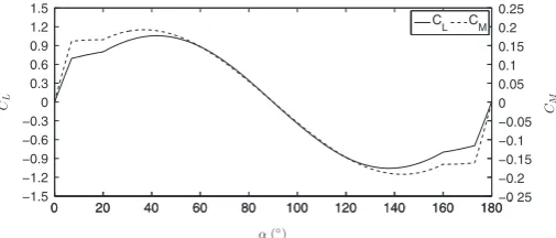
While it is clear that asymmetric plates held about an axis perpendicular to the flow should autorotate, this is not the case for symmetrical plates. Consider the steady lift and moment coefficient as shown inFig. 1. As the angle of attack,α, slowly increases, the lift force and torque increase until the plate begins to stall. At the stall point, these values decrease and eventually become insignificant when the plate is perpendicular to the flow. As the plate continues to rotate from 901to 1801, the cycle is repeated with reversed sign on the moment and lift. Therefore assuming a quasi-steady behaviour (i.e. that the plate is rotating so slowly that the aerodynamic forces at a given angle of attack can be assumed to be the static plate equivalents), a symmetrical plate exposed to a steady air stream would be expected to experience equal accelerating and retarding torque during different halves of the cycle, resulting in a static plate at the stable α¼901position, with no autorotation.

Smith (1971)experimentally investigated the autorotation of symmetrical wings about a span-wise axis perpendicular to the flow. Smith observed that in practice, a wing released from rest at an angular position at which the flow was stalled would come to rest (after a number of oscillations) in a statically stable position with the wing perpendicular to the free stream. However, if the wing was released at a small enough initial angle of attack,_αo, so that the flow was not stalled, the

wing usually began autorotating with the final direction of rotation determined by the initial orientation. Smith also reported that the wing would not autorotate if its moment of inertia,I, was too low. In this case it was unable to store enough angular momentum to pass through the stalled portion of its cycle, during which it received a retarding torque.

Smith (1971)found autorotation to be sensitive to the Reynolds number. Other factors influencing the rate of autorotation about an axis perpendicular to the flow are plate thickness, plate aspect ratio, lift and drag coefficients and the moment of inertia (Lugt, 1983).

Fig. 2shows the dimensions and orientation of the plate in all that follows. To account for the influence of plate thickness ratio,τ¼t=c, and aspect ratio,A¼b/c,Iversen (1979)obtained the correlation functions for tip speed ratio (TSR),Υ, based on data from experiments byBustamante and Stone (1969),Smith (1971)andGlaser and Northup (1971):

Υ¼V

U ¼f1ð ÞAf2ð Þτ; ð1Þ

whereVis the speed of the tip of the plate andUis the speed of the incoming air, while the functionsf1ðAÞandf2ðτÞare

defined as

f1ð Þ ¼A

A 2þð4þA2_Þ1=2

" #

2 A

Aþ0:595

0:76

" #

( )2=3

; ð2Þ

Fig. 1.Steady-state curves showing the variation of lift,CL, and moment,CM, coefficients with angle of attack,αfor static square flat plates held in a uniform steady flow (ESDU, 1970).

and

f2ð Þ ¼τ 0:329 ln

1

τ 0:0246 ln 1 τ

2!

: ð3Þ

The experiments upon which the correlations were derived involved plates of aspect ratios, 0:25rAr4, and thickness ratios, 0:0054rτr0:5. According toIversen (1979), for plates with aspect ratio,A45, the influence ofAon TSR can be ignored. The thickness ratio was also found to have a negligible effect on TSR for values less than 0.01 (Lugt, 1983).Smith (1971)performed his experiments at near constant values of a moment of inertia parameter,K, defined as

K¼ Iyy

ρc4_b; ð4Þ

whereρis the density of the air. Now, the moment of inertia,Iyyfor a flat plate, rotating about they-axis as shown inFig. 2,

is

Iyy¼ρpcbt c2

12þ t2

12

; ð5Þ

whereρpis the density of the plate. Substitution of Eq.(5)into Eq.(4), gives

K¼ 1

12 ρp

ρ t cþ

t3

c3

; ð6Þ

which, whenτ¼t=co1, results in

KC τ 12

ρp

ρ; ð7Þ

which means that for a constant density, thin plate,Kand_τare essentially the same parameter.

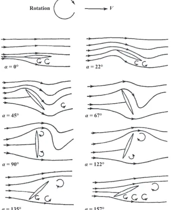
In his experiments,Smith (1971)observed a distinctly different flow pattern during autorotation, compared to the flow over a static plate (Fig. 3). The main difference being that the wing stalled much later than in the static case and the flow reattached later to the lower surface. As a result of this delayed stall, in the first 90₁cycle, positive lift and moment were increased while the negative lift and moment during the second half of the cycle were reduced by the delayed reattachment. The net driving torque created by this delayed stall phenomena gradually led to an increase in the wing's angular velocity until a steady average angular velocity was reached at which the average torque was reduced to zero by aerodynamic damping effects.

Smith (1971)went on to speculate that there were two possible causes for the delayed stall. First, he argued that the boundary layer on the upper (suction) surface of the wing takes time to thicken and separate when the angle of attack is rapidly increasing, such that the wing can reach a higher angle of attack before it stalls. Second, the flow over the upper surface of a wing with a rapidly increasing angle of attack is accelerating–this reduces the adverse pressure gradient thereby delaying stall. It is this hysteresis in the lift, resulting from unsteady aerodynamic effects, that causes autorotation.

Bustamante and Stone (1969),Iversen (1979)andSmith (1971)suggested that these unsteady aerodynamic effects could themselves be attributed to the large vortex shed from the retreating face of the plate which then creates an aerodynamic torque supporting autorotation due to the low pressure at its core. The sketch inFig. 4from a smoke-tunnel photograph of streak lines around an autorotating plate (Yelmgren, 1966) shows this large vortex that remains attached and is eventually shed from the retreating face of a rotor while no similar vortex is visible from the advancing face.

In addition to experimental investigations of plate autorotation, a number of 2D numerical studies of plate autorotation about a horizontal axis perpendicular to the flow in a steady uniform flow have been carried out, includingLugt (1980),

Seshadri et al. (2003),Mittal et al. (2004)andAndronov et al. (2007). These studies involve solving the 2D Navier–Stokes equations to obtain the unsteady flow field around an autorotating plate and the aerodynamic forces resulting. Early simulations byLugt (1980)were compared against experiments bySkews (1990), showing good agreement.

Other 2D numerical studies have also recently been conducted with a focus on understanding the aerodynamics of related problems such as the motion of falling paper (Andersen et al., 2005;Jin and Xu, 2008) and the aerodynamics of insect flightWang (2005). These studies focused on autorotation of high aspect ratio plates, exhibiting 2D motion, in low Reynolds number flow. The only low aspect ratio studies performed, such asDong et al. (2006)andTaira and Colonius (2009), relate to the aerodynamics of plates undergoing prescribed rotations such as those involved in insect flight as opposed to the non-linear flow involved in autorotation.

1.2. The context for the present study

It has been established for some time that wind borne debris accounts for a large proportion of building envelope failures during severe storms (Minor, 1994). While the initial failure of roof tiles and cladding may be due to extreme pressures, it is the subsequent flight of this debris and its impact on downwind buildings that causes much subsequent envelope failure. This was seen clearly during the Birmingham Tornado in the UK in 2005 (Marshall and Robinson, 2006).Holmes (2010)

refers to this wave of destruction as the“debris damage chain”, although it was first identified byMinor and Beason (1976)

clear focus byKatsura et al. (1992)who pointed out that 23% of the reported 63 fatalities during Typhoon Mireille which struck Japan in 1991 were caused by flying debris.

Tachikawa (1983)was one of the first to realise the importance of wind borne debris and presented both experimental data and analytical models in his paper. Following Tachikawa's work, a large number of models, all of them analytical, have been developed to predict the trajectories of plates in high winds (Holmes, 2004;Baker, 2007;Richards et al., 2008;Kordi and Kopp, 2009). Based on the principle of conservation of the linear and angular momentum, these models have relied on experimentally derived static plate force coefficients, which have been modified with Magnus force coefficients in order to take into account the autorotation. While the Magnus effect used in these analytical force models does account for the mean lift coefficient caused by the plate's autorotation, these models fail to account for the complex interactions that the plate makes with its wake, which have an effect on the fluctuating components of the force and moment coefficients.

The authors have already demonstrated (Kakimpa et al., 2010,2012a,b) how fully coupled Computational Fluid Dynamics (CFD) and Rigid Body Dynamics (RBD) models can be used to study the flight of plate debris. The cases of static plates, forced rotating plates, autorotating plates and free-flight simulations were discussed in this paper. While important from the point of view of providing validation evidence for the CFD modelling, the static and forced rotation cases are of limited value when modelling the actual flight of debris. This paper concentrates purely on the autorotation case.

The numerical model used for the autorotation is described inSection 2, followed by, inSection 3, the validation of the model against the experimental findings ofMartinez-Vazquez et al. (2010). This includes a demonstration of how the CFD predictions were able to offer insights into systematic experimental errors. Then, inSection 3.6, there follows a discussion of the complex flow fields seen during a cycle of autorotation and how these relate to the pressure, forces and moments acting on the plate. Finally, inSection 4, the validated model is used to revisit the correlation ofIversen (1979), Eqs.(1)–(3).

2. Numerical model

2.1. Coupled CFD_–RBD model

As part of the larger project to model the free flight of debris, a six degree of freedom (6DOF) rigid body dynamics (RBD) solver was incorporated into the ANSYS Fluent (Version 12.1) software, via User-Defined Functions. This coupled CFD–RBD model is described in detail inKakimpa et al. (2010). For fixed-axis autorotation, the RBD model essentially reduced to a single degree of freedom solver:

Iyy dωy

dt ¼My;

whereIyyis the mass moment of inertia,Myis the applied aerodynamic torque andωyis the angular velocity about theY

axis. The aerodynamic forces acting on the plate are computed from the static pressure and skin friction from the CFD solution and used to compute the aerodynamic torque,My, about the plate's geometric centre.

Unsteady Reynolds-Averaged Navier–Stokes (URANS) turbulence modelling was used throughout, together with a two-layer enhanced wall function approach. Large-Eddy Simulations (LES) would have been prohibitively expensive and second, URANS had proved accurate when modelling static and forced rotating plates in Kakimpa et al. (2010). The Realizable k-εturbulence model (Shih et al., 1995) was identified during that study to be the most accurate of the various RANS variants for this application and its use was continued in the present work. Verification of the CFD simulations (mesh independence, differencing schemes, etc.) is not discussed herein but may be found in earlier studies (Kakimpa et al., 2010).

2.2. Mass eccentricity submodel

Mass eccentricity is a term used to refer to the offset of the plate's centre of mass from the geometric centre of the plate. In most practical configurations, the axis of rotation corresponding to the plate's geometric centre-line does not run through the plate's centre of mass, generating an additional torque. A mass eccentricity model is incorporated in order to account for the effects of this additional eccentricity torque on the rotational motion of the plate.

Assuming a mass eccentricity error,e, during autorotation the plate would experience an additional torque,Te, about its

geometric centre line given by

Te¼mgesinαy; ð8Þ

wheremis the mass of the plate,gis gravitational acceleration, andαyis angle of the plate about theYaxis. In addition,

using the parallel-axis theory, the mass moment of inertia of the ideal plate,Iyy, would be corrected according to

Inyy¼Iyyþme2; ð9Þ

2.3. Bearing friction submodel

Previous experimental studies of plate autorotation (Iversen, 1979; Martinez-Vazquez et al., 2010) had indicated a significant contribution of bearing friction to the autorotational results. A friction torque for each bearing,Tfric, is included, in

addition to the aerodynamic and mass eccentricity torques:

Tfric¼ _jω

ωj

0:5μrd

ffiffiffiffiffiffiffiffiffiffiffiffiffiffiffiffiffiffiffiffiffiffiffiffiffiffiffiffiffiffi_ð

mgLÞ2_þD2 q

; ð10Þ

whereLis the aerodynamic lift force,Dis the aerodynamic drag force,ωis the rotational speed about the axis of rotation,d is the bore diameter of the bearing block andμris the rolling friction coefficient of the bearing block. The friction torque is

pre-multiplied byω=jωjso as to ensure that it always acts in the direction opposite to the plate's instantaneous direction of rotation.

3. Model validation

3.1. Experimental details

A full treatment of the experiments conducted in the wind tunnel at The University of Auckland, New Zealand, is given in

Martinez-Vazquez et al. (2010). A brief review is presented here in order to put the numerical modelling into context. The test sheet was a piece of expanded polystyrene, 1 m square, 0.0254 m thick and weighed 2.7 kg. Twenty-four differential pressure transducers and associated data loggers were mounted inside the sheet as seen in Fig. 5(a). The differential pressure transducers were mounted with one pressure tap directly opposite the other on the reverse side of the sheet. During the autorotation experiments the sampling rate was set to 200 Hz, which approximates to a data sample every 21at the autorotation rates seen in the experiments.

In the wind tunnel, air was blown through a 3.5 m square nozzle towards an open area for testing at speeds of 5, 7.5 and 10 m s1_{. Two frames held the sheet in place, with roller bearings to allow for the free rotation of the plate. The plate was}

released from an initial angle of attack of 151to the horizontal to ensure the board entered autorotation. Only the last 30 s of each run were analyzed, once stable autorotation had established itself. The computation of forces and moments was

Fig. 5. Distribution of sensors and data loggers inside the Auckland test sheet (Martinez-Vazquez et al., 2010).

58 59 60 61 62 63 64 65 66 67 68 −0.2

−0.1 0 0.1 0.2 0.3

Time (s)

CM

Raw Experimental Data Filtered Experimental Data

achieved by integrating the net pressure coefficients, found from the differential pressure transducers. An onboard gyroscope was used to calculate the instantaneous angular velocity of the plate.

3.2. Data analysis

There was evidence from the raw data of the moment coefficient,CM, that the time series consisted of several harmonics.

Fig. 6shows a short segment of the moment coefficient for the raw and filtered experimental data for 5 m s1_{case. To test}

this, the harmonics ofCMwere found using a Discrete Fourier Transform (DFT) algorithm based onFrigo and Johnson (1998).

The DFT was used to compute the frequency domain representation of the experimental time-series. The raw experimental signal was first de-trended in order to remove any linear static components such as those due to average autorotational lift. Frequency filtering was then performed and the signal was then re-constructed as a complex-periodic signal using only the dominant harmonic frequencies. For a signalx(t) containing a sequencefxngof uniformly spaced time measurements of non-dimensionalised moment coefficient,CM, the exact equivalent of a discrete Fourier Transform,Xk, is computed as

Xk¼ ∑ N1

n¼0

xnei2πkn=N k¼0;1;2;…ðN1Þ; ð11Þ

whereNis the number of elements in the raw signal sequence.

The frequency,f, amplitude,A, and phase,ϕ, are then obtained from the DFT,Xk, according to

fi¼ i NΔt

Ai¼ 2jXkðiÞj

N ϕi¼argðXkðiÞÞ

9 > > > > > = > > > > > ;

i¼0;1;2;…;ðN1Þ: ð12Þ

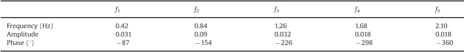
The frequency–amplitude signal generated from the raw experimental data, shown inFig. 7, shows that the raw signal is predominantly complex-periodic, consisting of five major harmonics whose frequencies are all integral multiples of the first harmonic frequency,f1¼0.42.Table 1shows the amplitude, frequency and phase information for the harmonics.

The first peak corresponds to the frequency of rotation of the peak,f1¼1=T, whereTis the period of rotation. For the

5 m s1_{case,Martinez-Vazquez et al. (2010)quote the period as 2.36 s, which gives a value off}

1¼0.424, which is very close

to those produced by the DFT here. The second peak corresponds to the vortex shedding phenomenon, which occurs twice in each cycle. The third, fourth and fifth harmonics were, at this point, unaccounted for but are accounted for by the (as yet unidentified) effects of mass eccentricity (seeSection 3.5). Also, the five main peaks exhibit side lobes, normally associated with frequency leakage and the presence of which is governed either by the choice of window function or the length of the time series used.

Using the harmonic frequencies and their corresponding amplitude and phase information, a sine wave reconstruction of the original signal was computed. Given n number of harmonics, in this case 5, each with a frequency, fi, that has a

corresponding amplitude Ai, and phase ϕi, the filtered time-series y was computed as a combination of n sine waves

0 0.2 0.4 0.6 0.8 1 1.2 1.4 1.6 1.8 2 2.2 2.4

0 0.02 0.04 0.06 0.08 0.1

f (Hz)

Amplitude

Raw Expt Data Filtered Expt Data

Fig. 7.Frequency domain representations of raw and reconstructed time series of experimental moment coefficient,CM.

Table 1

Frequency, amplitude and phase information computed for the five major harmonic frequencies,f1–f5, of the raw experimental data from the Auckland tests.

f1 f2 f3 f4 f5

Frequency (Hz) 0.42 0.84 1.26 1.68 2.10

Amplitude 0.031 0.09 0.032 0.018 0.018

according to

y¼ ∑n

i¼1

Ai sinð2πfitþϕiÞ i¼0;1;2;…;n; ð13Þ

wheretis the time. In addition to the raw data,Fig. 6shows a segment of the complex periodic reconstruction of the signal using frequency and amplitude data from Table 1. Fig. 7 also shows the good agreement between the frequency representations of the raw experimental time signal and the reconstructed time signal.

3.3. The Auckland model

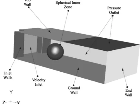
The Auckland domain is shown schematically inFig. 8and was designed to replicate the flow conditions within the wind Auckland wind tunnel as closely as possible. A rigid, spherical inner zone containing the plate is free to rotate. The outer zone is kept stationary throughout. The two zones are connected via a non-conformal sliding mesh interface–commonly used when modelling turbomachinary using CFD–which can be seen inFig. 9. The mesh was entirely block-structured and consists of 291 000 cells, with boundary layers grown away from the walls of the plate.

A square, flat plate of mass,m, 2.7 kg, side length,c,b, 1 m and thickness,t, 0.0254 m was used, with an initial angle of attack of 101. The inlet was modelled as a constant velocity boundary while the outlets were modelled as constant pressure boundaries. At the inlet, 1% turbulence intensity and 0.02 m turbulence length scale were specified, corresponding to typical

Fig. 8.Domain corresponding to the wind tunnel experiments ofMartinez-Vazquez et al. (2010).

low turbulence wind tunnel values fromESDU (1970). Three cases were run with mean wind speeds,Uw, of 5.0 m s1, 7.5 m s1

and 10.0 m s1_{, corresponding directly to the wind speeds used in the experiments. Three outlet boundaries were required,}

corresponding to both the sides and the far section of the top boundary–the plate was mounted in an open working section. The inlet is a 3.5csquare while the test section is 15c7c3:5c. The plate's axis of rotation is 5cfrom the inlet and 1.2cfrom the bottom wall. The top wall stretched for 8cfrom the inlet before giving way to the top outflow boundary.

3.4. Calibration

As a preamble to the calibration process, it should be noted that a cuboid domain was initially used, with the plate far from the walls, with a low blockage ratio. Using this domain and the same set-up as just described, the CFD simulations produced aCM, which had only two harmonics, each at more than double the frequencies seen experimentally in the

Auckland wind tunnel. At this point, a number of possibilities for the lack of a complex harmonic response were considered:

With the Auckland domain and a perfectly balanced, friction free plate, the CFD model predicted a shift in the angular velocity of the plate as compared with the Cuboid domain. The frequencies of the first two harmonics were reduced relative to the Cuboid domain and coincided more closely with those peaks for the raw and reconstructed data inFig. 7. However, the third, fourth and fifth harmonics ofFig. 7are missing from the Auckland domain simulations. The reduction in the angular speed of the plate for the Auckland domain was attributed largely to the asymmetry introduced into the flow field due to the close proximity of the floor to the plate.

3.5. Mass eccentricity

Using the Auckland domain, a submodel was incorporated into the RBD solver for the plate which would account for mass eccentricity. While the experimentalists had taken all possible steps to keep the mass distribution symmetrical within the instrumented plate, it was postulated that there was a degree of mass eccentricity, which would account for the missing harmonics ofFig. 7. The model used here is based on an assumption that in the experimental setup of the plate, small errors of up to 5% of the plate's length may occur while positioning the plate's centre of mass. Such errors would be expected due to the complexity of the data acquisition and plate mounting and support system used (Martinez-Vazquez et al., 2010).

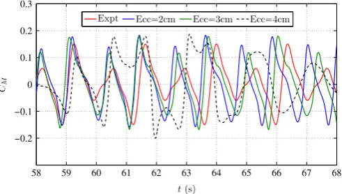
The CFD simulations indicated that low values of mass eccentricity error of 0.02 m and 0.03 m have the effect of accelerating the plate through one half of its cycle, followed by a deceleration in the second half. For values of greater than 0.04 m, the eccentricity torque effectively prevents the plate from entering the autorotating state.Fig. 10 shows the time series of the computed moment coefficient,CM, for eccentricity errors of 0.02, 0.03 and 0.04 m compared with the reconstructed experimental

time series. In each case, the dominant frequency appears to be dependent on the eccentricity error. With an eccentricity error of 0.04 m, the time series shows a strikingly different pattern to the lower eccentricity errors. This is because at this size of error, the plate is only just capable of maintaining autorotation. Indeed, inFig. 10, the envelope of the moment coefficient exhibits a beating pattern, which sees the amplitude of the moment coefficient falling to zero for periods.

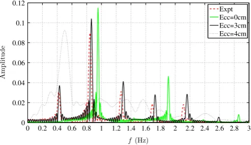
In the frequency domain,Fig. 11shows that a value of the mass eccentricity error of 0.03 m offers the closest match to the reconstructed experimental data in terms of both the number of harmonics present but also the frequencies of those harmonics. The frequency response of the case with mass eccentricity of 0.04 m is far from the reconstructed experimental data and again shows that the fine tuning of the mass eccentricity error is crucial to the success of this validation process.

It was found that even with unphysically large values of bearing friction, there was an insignificant change in the response of the autorotating plate and so this was discounted as a source of the complex harmonic behaviour.

3.6. Surface pressures and flow features

With the Auckland domain and the mass eccentricity sub-model, the CFD model was compared against the large amounts of experimental surface pressure data that were available. The 24 differential pressure taps ofFig. 5each measured the instantaneous differential (net) pressure between a point on the front of the plate and one at the same location on the rear of the plate. For purposes of comparison, the CFD model produced static pressure values at each of the 1600 faces on the front and rear faces of the plate. So, some manipulation was required to produce the differential pressures at the sensor locations. A normalisation is used to produce the net pressure coefficient:

CNP¼

PifrontP

i

rear

0:5ρU2w ;

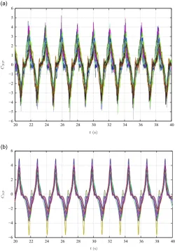
wherePifrontis the static pressure on the front face at the position of theith sensor andUwis the wind speed.Fig. 12(a) shows

the time series of the net pressure coefficient for the experiments and the CFD simulations, plot (b), at all the locations of the sensors for the case with a wind speed of 5 m s1_{. Qualitatively, the two sets of time series data look similar, but it is not}

until a single cycle is analysed that the extent of the agreement is shown.

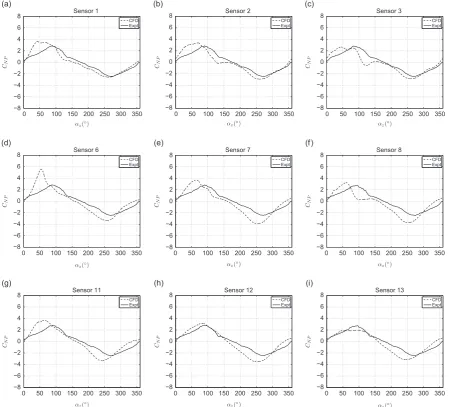
To this end,Fig. 13shows the experimental data, which has been averaged over a larger number of cycles, compared with the CFD predictions of the normal pressure coefficient from a single cycle (each cycle is identical because of the deterministic nature of the simulations). This subset of sensor locations were chosen for the plot because they provide a subset that captures some of the more dominant fluid dynamics processes associated with autorotation. For example, sensors 1, 2, 3 are located close to the advancing (or retreating, depending on the position within the cycle) edge and could capture pressure effects associated with the retreating edge vortices.

Again, qualitatively, the results look similar but there are some sensors near the side edges of the plate (e.g. sensor 6), where the CFD simulations predict significantly larger peak pressures. This may be attributed to the inaccurate representation of vortex core pressure by the Unsteady Reynolds-Averaged Navier–Stokes (URANS) models, which do not resolve the flow structures but rather represent their gross statistical properties. Alternatively, these discrepancies might arise from the close proximity of the plate's support frame in the experimental set-up, which may have disrupted the flow near these edges and weakened the large edge vortices.

The accurate prediction of the surface pressure distribution is crucial for making predictions about the flight of windborne debris. An accurate prediction of the surface pressure allows for an accurate prediction of the location of the centre of pressure and thence the aerodynamic torque acting on the plate.Figs. 14and15show the numerical static pressure coefficient distributions:

CP¼ P 0:5ρU2w

;

on the front (windward) and rear (wake facing) faces of the plate– the nomenclature for a plate autorotating in the clockwise sense is shown inFig. 2. It should be noted that the results presented here are for a stably autorotating plate and represent the instantaneous pressure coefficients at given angles of attack,αy, during a single cycle.

Visualisation of the flows around the plate are challenging, but a useful quantity is the Q-value or Q-criterion. For incompressible flow theQ-value, an objective method of vortex identification proposed byHunt et al. (1988), is computed as

Q¼1 2 jΩj

2_jSj2

;

where

Ω¼1

2 ∇Uð∇UÞ T

h i

;

is the vorticity tensor and

S¼1

2 ∇Uþð∇UÞ T

h i

;

is the strain-rate tensor. TheQ-criterion (Hunt et al., 1988) identifies a vortex as a region whereQ40 such that flow swirl, represented byjΩj, is more prominent than flow shear, represented byjSj. This method of vortex identification has been preferred over vorticity magnitude since vorticity has been shown not to distinguish between pure shearing motions and the actual swirling motion of a vortex (Kolar, 2007).Fig. 16should be used in conjunction with the two pressure plots, showing as it does both the orientation of the plate and the contours of the Q-value on a vertical plane through the centreline of the plate. In addition,Fig. 17(a) and (b) will be referred to in the following discussion–this figure shows that theQ¼10 s1_{isosurface for the square plate used in the base case inSection 4. Although a slightly different set-up (a large}

rectangular domain and no mass eccentricity model), the flow field closely resembles that seen in the Auckland simulations. On the front, windward face, a large, positive stagnation pressure is seen close to the advancing edge (bottom edge) of the face inFig. 14, particularly for 301oαyo1201. Atαy¼901, a central location for the stagnation point would be seen–in the autorotating case, the rotation of the plate means that the relative velocity of the plate to the wind increases near the advancing edge, resulting in the increased static pressure seen in this location (towards the bottom of Fig. 14(d), for example). Atαy¼01, there is no negative pressure region for the rotating plate, which would be seen for a static plate where flow separation takes place at the sharp upstream corner of the plate.

Meanwhile on the rear, wake facing face (Fig. 15), the presence of tip (or, more sensibly with this aspect ratio, side) vortices manifests itself as areas of negative pressure along the side edges (left and right edges) of the face–particularly

20 22 24 26 28 30 32 34 36 38 40

−6 −5 −4 −3 −2 −1 0 1 2 3 4 5 6

20 22 24 26 28 30 32 34 36 38 40

−6 −4 −2 0 2 4 6

when 301oαyo901. In particular, for the caseαy¼901,Fig. 17(b) shows the presence of these tip vortices, which can be seen forming as the air flows around the vertical sides of the plate. (The wind is blowing from top right to bottom left, aligned with thex-axis, in all plots inFig. 17.) Simultaneously at the retreating edge, another vortex is forming creating negative pressure regions close to the retreating edge (the top edge of the rear face). A retreating edge vortex can be seen developing inFig. 17(b) and also inFig. 16(b)–(e), until finally being shed inFig. 16(f) forαy¼1501. Further on still in the cycle, at αy¼01ð ¼1801Þ,Fig. 17(a) shows the remnants of the retreating edge vortex as it moves away from the plate (interestingly still attached to the tip vortex tubes). Later still, the second retreating edge vortex inFig. 17(b) is the one that was developed and shed in the previous cycle.

There are some similarities between the vortices ofFig. 16and the sketch ofSmith (1971)(Fig. 3). Atαy¼01, the small vortices below the plate can be seen, but these appear to have disappeared in the CFD simulation whenαy¼301, when Smith suggests they are still present. The other main feature, the retreating edge vortex is present in both studies. The numerical results indicate a thin, stretched vortex downstream of the advancing edge, which could be interpreted as the two or three smaller vortices that Smith has in this position.

The negative pressure from the wake flow structures, together with the positive stagnation pressure at the front of the plate create the positive net pressure distribution coefficient, is shown in Fig. 18. As illustrated in Fig. 18(a)–(d), for 0_1rαyr901the net pressure in the top half of the plate is much greater than the net pressure in the bottom half, resulting in a positive accelerating torque. Beyondαy901however,Fig. 18(e) and (f), the net pressure in the bottom half of the plate is greater than the net pressure in the top half of the plate, creating a decelerating torque. It is this balance of positive and negative torques during the various stages of the cycle that determines whether the plate will stably autorotation or not.

0 50 100 150 200 250 300 350

−8 −6 −4 −2 0 2 4 6

8 Sensor 1 _CFD

Expt

0 50 100 150 200 250 300 350

−8 −6 −4 −2 0 2 4 6

8 Sensor 2

CFD Expt

0 50 100 150 200 250 300 350

−8 −6 −4 −2 0 2 4 6

8 Sensor 3

CFD Expt

0 50 100 150 200 250 300 350

−8 −6 −4 −2 0 2 4 6

8 Sensor 6

CFD Expt

0 50 100 150 200 250 300 350

−8 −6 −4 −2 0 2 4 6

8 Sensor 7

CFD Expt

0 50 100 150 200 250 300 350

−8 −6 −4 −2 0 2 4 6

8 Sensor 8

CFD Expt

0 50 100 150 200 250 300 350

−8 −6 −4 −2 0 2 4 6

8 Sensor 11

CFD Expt

0 50 100 150 200 250 300 350

−8 −6 −4 −2 0 2 4 6

8 Sensor 12

CFD Expt

0 50 100 150 200 250 300 350

−8 −6 −4 −2 0 2 4 6

8 Sensor 13

CFD Expt

4. Iversen correlations

The correlations that were derived by Iversen (1979) have stood the test of time, albeit with very few researchers working in this area. By using the validated CFD–RBD model, this section investigates the validity of the correlations over a range of aspect ratios, thickness ratios and values of the moment of inertia parameter,K. A sensitivity study is used, centred around abase case, which will itself be described and analysed in detail.

Face2 Pressure

−0.5 −0.4 −0.3 −0.2 −0.1 0 0.1 0.2 0.3 0.4 0.5

−0.5 −0.4 −0.3 −0.2 −0.1 0 0.1 0.2 0.3 0.4

0.5 Face2 Pressure

−0.5 −0.4 −0.3 −0.2 −0.1 0 0.1 0.2 0.3 0.4 0.5

−0.5 −0.4 −0.3 −0.2 −0.1 0 0.1 0.2 0.3 0.4 0.5 Face2 Pressure

−0.5 −0.4 −0.3 −0.2 −0.1 0 0.1 0.2 0.3 0.4 0.5

−0.5 −0.4 −0.3 −0.2 −0.1 0 0.1 0.2 0.3 0.4

0.5 Face2 Pressure

−0.5 −0.4 −0.3 −0.2 −0.1 0 0.1 0.2 0.3 0.4 0.5

−0.5 −0.4 −0.3 −0.2 −0.1 0 0.1 0.2 0.3 0.4 0.5 Face2 Pressure

−0.5 −0.4 −0.3 −0.2 −0.1 0 0.1 0.2 0.3 0.4 0.5

−0.5 −0.4 −0.3 −0.2 −0.1 0 0.1 0.2 0.3 0.4

0.5 Face2 Pressure

−0.5 −0.4 −0.3 −0.2 −0.1 0 0.1 0.2 0.3 0.4 0.5

−0.5 −0.4 −0.3 −0.2 −0.1 0 0.1 0.2 0.3 0.4 0.5

4.1. Base case

The choice of parameters for the base case was based on the Auckland experiment setup. A new cuboid domain, however, was constructed to give the results the generality of a uniform cross-section wind tunnel. Here the same spherical inner region as used in the validation process was contained within a domain of dimensions 13:5c7c7c

Face1 Pressure

−0.5 −0.4 −0.3 −0.2 −0.1 0 0.1 0.2 0.3 0.4 0.5

−0.5 −0.4 −0.3 −0.2 −0.1 0 0.1 0.2 0.3 0.4

0.5 Face1 Pressure

−0.5 −0.4 −0.3 −0.2 −0.1 0 0.1 0.2 0.3 0.4 0.5

−0.5 −0.4 −0.3 −0.2 −0.1 0 0.1 0.2 0.3 0.4 0.5 Face1 Pressure

−0.5 −0.4 −0.3 −0.2 −0.1 0 0.1 0.2 0.3 0.4 0.5

−0.5 −0.4 −0.3 −0.2 −0.1 0 0.1 0.2 0.3 0.4

0.5 Face1 Pressure

−0.5 −0.4 −0.3 −0.2 −0.1 0 0.1 0.2 0.3 0.4 0.5

−0.5 −0.4 −0.3 −0.2 −0.1 0 0.1 0.2 0.3 0.4 0.5 Face1 Pressure

−0.5 −0.4 −0.3 −0.2 −0.1 0 0.1 0.2 0.3 0.4 0.5

−0.5 −0.4 −0.3 −0.2 −0.1 0 0.1 0.2 0.3 0.4

0.5 Face1 Pressure

−0.5 −0.4 −0.3 −0.2 −0.1 0 0.1 0.2 0.3 0.4 0.5

−0.5 −0.4 −0.3 −0.2 −0.1 0 0.1 0.2 0.3 0.4 0.5

with the centre of mass of the plate positioned 3.5cfrom the inlet, bottom, top and side boundaries. When the angle of attack, αy, is 7901, the blockage ratio is 2%. The bottom, top and side boundaries were modelled as smooth wall

boundaries. The velocity inlet was given the same turbulence intensity and length scale as before.

The base case setup is listed in Table 2, where the associated non-dimensionalised parameters are also presented. The value ofKis at the low end of those seen in the various sets of experiments thatIversen (1979)based his correlations on. The low value is due to the low density of the polystyrene plate as compared with the metal plates used in many of the experiments thatIversen (1979)analyzed.

All the cases described were run for a long enough period to allow them to reach a state of stable autorotation. This time varied according to the mass moment of inertia,Iyyof the plate and so was hard to predict accuratelya priorihow long each

run would require. So, some monitoring of the response of the angular velocity was required.Fig. 19shows the response of ωyfor the base case run. As can be seen from the figure, the stable autorotation is reached by the fourth cycle–here the time

to stable autorotation is short because of the low mass moment of inertia of the base case plate. The other case shown in

Fig. 19is for a case with four times the density of the base case plate (hence its moment of inertia parameter,K¼4KB, where KBis the base case moment of inertia parameter).

Once stable autorotation was reached, three complete cycles (between four of the peaks inFig. 19) of theωyresponse

frequency of the variation of theωysignal:

Ωy¼

2πðnp1Þ

Δtðjnpj1Þ;

ð14Þ

wherenpis the number of peaks used (here 4),Δtis the time step used in the CFD simulations andj1andjnp are the integer locations of the first andnth

p peaks in the time signal. Since the plate goes through two cycles of vortex shedding every time it completes a full rotation, it is expected thatΩy¼2ωy, which is indeed that case for all cases investigated. For the base case, ωy¼3:11 rad s1andΩy¼6:22 rad s1.

Fig. 20shows the variation of the angle of attack, angular velocity and the force and moment coefficients over one of these half rotations, for the base case. In the figure, the half cycle extends from the moment at which the angle of attack is 01 round to when it is 180₁. At the start of the cycle, the angular velocity is at a minimum, following on from a period of negative, decelerating moment at the end of the previous cycle, plot (d). Then, as the plate presents more of its surface area to the oncoming flow, the drag and lift forces (inferred from their coefficients) increase, resulting in a positive, accelerating moment acting on the plate, which itself peaks at approximately 451into the cycle. The plate's angular momentum peaks at an angle of attack of approximately 901, as the moment coefficient moves from positive to negative. This cycle then repeats as the plate passes through its starting position.

As seen previously inSection 3.6,Fig. 17(a) and (b) shows theQ¼10 s1

downstream. InFig. 17(a) the vortex is still attached by two side vortex tubes. Also seen are two vortex“legs”which are caused by vortices being shed from the tips (or sides) of the plate and being carried downstream.

4.2. Sensitivity to moment of inertia parameter

WhileIversen (1979)was able to produce and test the correlations of tip speed ratio,Υ, for aspect ratio and thickness ratio (Eqs.(2) and (3)), he was less committal in producing one for the moment of inertia parameter,K. In his paper, it was

Differential Pressure (F2−F1)

−0.5 −0.4 −0.3 −0.2 −0.1 0 0.1 0.2 0.3 0.4 0.5

−0.5 −0.4 −0.3 −0.2 −0.1 0 0.1 0.2 0.3 0.4

0.5 Differential Pressure (F2−F1)

−0.5 −0.4 −0.3 −0.2 −0.1 0 0.1 0.2 0.3 0.4 0.5

−0.5 −0.4 −0.3 −0.2 −0.1 0 0.1 0.2 0.3 0.4 0.5

Differential Pressure (F2−F1)

−0.5 −0.4 −0.3 −0.2 −0.1 0 0.1 0.2 0.3 0.4 0.5

−0.5 −0.4 −0.3 −0.2 −0.1 0 0.1 0.2 0.3 0.4

0.5 Differential Pressure (F2−F1)

−0.5 −0.4 −0.3 −0.2 −0.1 0 0.1 0.2 0.3 0.4 0.5

−0.5 −0.4 −0.3 −0.2 −0.1 0 0.1 0.2 0.3 0.4 0.5

Differential Pressure (F2−F1)

−0.5 −0.4 −0.3 −0.2 −0.1 0 0.1 0.2 0.3 0.4 0.5

−0.5 −0.4 −0.3 −0.2 −0.1 0 0.1 0.2 0.3 0.4

0.5 Differential Pressure (F2−F1)

−0.5 −0.4 −0.3 −0.2 −0.1 0 0.1 0.2 0.3 0.4 0.5

−0.5 −0.4 −0.3 −0.2 −0.1 0 0.1 0.2 0.3 0.4 0.5

Table 2

Parameter set for the base case.

Chord,c 1.0 m Width,b 1.0 m

Thickness,t 0.0254 m Density,ρp 106.3 kg m3

Mass moment of inertia,Iyy 0.225 kg m2

Aspect ratio,A 1.0

Thickness ratio,τ 0.0254 Mass moment of 0.1838

Wind speed,u 5 m s1

Inertia parameter,K

0 2 4 6 8 10 12 14 16 18 20 0

0.5 1 1.5 2 2.5 3 3.5 4 4.5 5

Fig. 19. Variation of the angular velocity,ωy, with time for the base case and for a case where the moment of inertia parameter is four times that of the base case.

0

1

2

3

4

5

0

45

90

135

180

0

45

90

135

180

1

2

3

4

5

0

45

90

135

180

−1

0

1

2

3

4

Drag

Lift

0

45

90

135

180

−0.2

−0.1

0

0.1

0.2

suggested that indeed,

Υ¼f1ðAÞf2ðτÞf3ðKÞ; ð15Þ

but the experimental evidence was complicated, since many of the experiments used quite different experimental arrangements.

As mentioned earlier, the base case has a value ofKthat was towards the bottom of the range considered by Iversen. A series of simulations with increasing values ofKwere conducted, simply by increasing the density of plate above its base case value.Fig. 21shows the variation of the mean, maximum and minimum values of_ΥwithK, in the style of Iversen's paper.1_{There is clearly an asymptotic relationship here, withΥtending to some constant value for largeK. The variation in} TSR during a cycle, as witnessed by the convergence of the maximum and minimum values, reduces as the moment of inertia of the plate increases. This is in agreement with Iversen's observations and those for the two simulations presented inFig. 19, where the case withK¼4KBhas an increased mean angular velocity with reduced variation in that variable.

Although this was not knowna priori, the value ofKused in the base case,KB, was only just above what Iversen called,

KM, the minimum value below which the inertia of the plate is not great enough to carry it through the retarding-moment

portion of the cycle (αy4901inFig. 20(d)). Indeed, a reduction inKto half its base case value resulted in damped oscillations and ultimately a plate that stuck at an angle of attack of 901, albeit with some minor oscillations back and forth.

The aspect and thickness ratios of the base case are in the centre of the range of values considered by Iversen when constructing his correlations. Therefore, making the assumption that Iversen's correlations forf1andf2hold, it is possible to

plotΥ=f1f2against Kin order to find a functional relationship forf3. For the base case plate geometry, regardless of its

density,f1¼0.4547 andf2¼0.8765, givingf1f2¼0:3985. It was found that the function

f3ðKÞ ¼aKð1bKexpcK ffiffiffiffi

K p

Þ ð16Þ

with aK¼0.9516, bK¼1.0487 and cK¼4.1307 and is used in Eq. (15) to produce the“Fit” curve in Fig. 21. If the CFD

simulations were following Iversen's correlations exactly, aKwould be unity –the fact that it differs from this slightly

indicates some numerical error. However, when considering the experimental data spread in Iversen's experimental database, this is an acceptable error.

4.3. Sensitivity to aspect ratio

In order to test the sensitivity of the simulations to aspect ratio,τ¼b=c, three extra inner, spherical domains were built and meshed. The new plates had aspect ratios of 0.5, 0.33 and 0.2, based on a chord of 1 m. These could be rotated through 90₁about thexaxis to give three further aspect ratios of 2, 3 and 5. However, this meant that only the cases withA_o1 had the same thickness ratio, since the plates all had a thickness,t, of 0.0254 m. Nonetheless, it seems reasonable to account for variations in the thickness ratio by assuming that Eq.(3)holds over the range under consideration.

Fig. 22shows the variation of the tip speed ratio,Υ, with aspect ratio,A, both according to the Iversen correlations, f1ðAÞf2ðτÞand for the numerical simulations. Two sets of results are shown, one set for the“Fixed density”plates, which had

the low density of the base case plate. Due to this constant density, the value ofKforAo1 was 0.184, but increased when

0 1 2 3 4 5 6 7

0 0.05 0.1 0.15 0.2 0.25 0.3 0.35 0.4 0.45 0.5

Moment of inertia parameter, K

Tip speed ratio,

ϒ

Average Fit

Minimum during cycle Maximum during cycle

Fig. 21.The variation of the tip speed ratio,Υ, with the moment of inertia parameter,K, for aspect ratio,A¼1 and thickness ratio,τ¼0:0254.

1

A₄1 because the thickness ratio,_τ, was not constant in this region. In order to isolate the results from a variation inK, a second set of simulations were run with a fixed value of K¼0.735, which is still towards the lower end of the range considered byIversen (1979).

In the range 0:5oAo2, the agreement with Iversen's correlations is encouraging. WhenA41, the TSR predicted by the numerical simulations is significantly larger than Iversen would suggest. The discrepancy increases with aspect ratio. These plates are rotating at angular velocities an order of magnitude greater than the base case plate, which might explain some of the inaccuracy. However, the time step used in the simulations was reduced accordingly, so that the rotation per time step would be approximately constant for all simulations. Rather, the sources of difference whenA41 could be due to the lack of bearing friction in the numerical simulations and the blockage ratio in the simulations, which was low compared with the experiments upon which Iversen's correlations were based.Fig. 17(d) shows theQ-criterion for theA¼2.0 plate. Here the very distinct vortex structures of the base case, plot (a) in the figure, are not as clear. The retreating edge vortex is still discernable, but the edge vortices seem to have been wrapped up in this vortex.

WhenAo1, the simulations again over-predict–by a factor of 1.5 for the very lowest aspect ratio considered. For these very slender plates, the vortices shed from around the long, chord-wise edges of the plate, may be interfering with the retreating edge vortex in a complex manner, which the numerical simulation is not capable of capturing accurately. There is not enough evidence here to suggest that Iversen's correlations break down at these low aspect ratios. The aspect ratio correlation is shown to work very well againstGlaser and Northup (1971), whereKC6 andτ¼0:03125. A number of tests were conducted in this range ofKandτ, but a similar trend was seen, with the tip speed ratio being higher than predicted

0 1 2 3 4 5 6

0 0.1 0.2 0.3 0.4 0.5 0.6

Aspect Ratio, A

Tip speed ratio,

ϒ

Iversen f 1 f2 Numeric, Fixed density Numeric, Fixed K

Fig. 22.The variation of the tip speed ratio,Υ, with aspect ratio,A, for plates of low and high moment of inertia parameter,K, as predicted by theIversen

(1979)correlations and the numerical simulations.

0 1 2 3 4 5 6 7

0 0.5 1 1.5 2 2.5 3 3.5 4

outside the range, 0:5oAo2.Fig. 17(c) shows theQ-criterion for theA¼0.5 plate, which bears a close resemblance to the plot for the base case. The long, side edges ensure that vortices shed from these locations compete with the retreating edge vortex and are clearly visible. The quite different flow fields whenAo1 andA41 tend to confirm the shape of Iversen'sf1

correlation, Eq.(2).

There is one anomalous point inFig. 22–for the low density plate withA¼0.33, the TSR does not lie in the expected position between the values forA¼0.2 and 0.5. This is because, for some unexplained reason, the variation in the angular velocity exhibits a complex period nature,Fig. 23–something that none of the other cases in this sensitivity study exhibit.

4.4. Sensitivity to Reynolds number

Using the base case configuration, four more wind speeds of 0.1, 0.25, 1, 10 and 20 m s1were simulated, corresponding to a range of chord Reynolds numbers from 6:9103 to 1:4106. Iversen used both“chord”and “thickness”Reynolds numbers, but here only the chord Reynolds number, Re¼ρuc=μ, is considered because the thickness ratio at each wind speed is constant. The range of Reynolds numbers chosen corresponds to those seen with flying debris. It should be noted that during the initial acceleration phase of the debris flight, the Reynolds numbers will be towards the top end of the range

104 ₁₀5 ₁₀6

0 0.05 0.1 0.15 0.2 0.25 0.3 0.35 0.4 0.45 0.5

Chord Reynolds number, Re

Tip speed ratio,

ϒ

Average

Minimum during cycle Maximum during cycle

Fig. 24.The variation of the tip speed ratio,Υ, with the Reynolds number, Re, for aspect ratio,A¼1, thickness ratio,τ¼0:0254 and moment of inertia parameter,K¼0.1838.

104 ₁₀5 ₁₀6

0 0.2 0.4 0.6 0.8 1

Chord Reynolds number, Re

Force coefficient

Drag Lift

considered here. As the plate approaches the wind speed, the Reynolds number, based on the relative velocity between the plate and the wind, will reduce, possibly by an order of magnitude.

For these plates with an aspect ratio of 1, with thef3ðKÞcorrelation used, the Iversen correlations would predictΥ¼0.31,

which, fromFig. 24, is the asymptotic value as Re becomes large. This concurs with the conclusion ofIversen (1979)that the “tip speed ratio is relatively independent of the Reynolds number”. For the lowest values of Re in this limited range, there is a rapid dropoff in tip speed ratio. Due to the low moment of inertia parameter of the base case plate, there is a large variation in angular velocity during each cycle (at all Reynolds numbers). However, for the lowest wind speed,u¼0.1 m s1

, this means that the plate is almost becoming stationary at certain points in each cycle, which clearly will result in a quite different flow regime than at higher wind speeds. It could therefore be postulated that there will be a finite Reynolds number below which the plate will no longer autorotate. Iversen, however, did not discuss this eventually, possibly because the plates he was analysing all had much higher values ofK.

The mean drag,CD, and lift,CL, coefficients over four cycles are plotted against chord Reynolds number inFig. 25. Again

there is an asymptotic limit for both force coefficients as Re increases above 105. Iversen found a slight functional dependence of the drag coefficient on the chord Reynolds number, but this was subject to a good deal of experimental scatter. The values ofCDthat Iversen quoted were between 0.8 and 1.2, so the values predicted by the simulations fall well

within that range.

4.5. Sensitivity to thickness ratio

The robustness of Iversen'sf2ðτÞcorrelation was tested by creating four plates with thicknesses from 0.01 to 0.2 m.

All other base case parameters were retained, except for the plate withτ¼0:01 m, where the density had to be doubled to get the plate to autorotate.Fig. 26shows that the values ofΥpredicted by Iversen (ieΥ¼f1ðAÞf2ðτÞf3ðKÞ, withf3ðKÞgiven by

Eq. (16)) in comparison with the numerical predictions. For the thickest plate, there is some deviation from the value predicted by Iversen. A close inspection of Iversen's data reveals a paucity of data above_τ¼0_:1. The data above this value was calculated using the wind tunnel data ofGlaser and Northup (1971)with a plate of aspect ratio,A¼0.5, and moment of inertia parameter,K, in the range 1.3–32, well above the range used in the numerical simulations.

5. Conclusions

This paper demonstrates that it is possible to model a complex fluid–structure interaction, such as autorotation, using Reynolds-Averaged Navier_–Stokes turbulence models. In particular, the use of Unsteady RANS turbulence models, coupled with a single degree of freedom solver, is indicated in this case, with predicted autorotation rates, moment coefficients and surface pressures comparing very well with experimental results. Indeed, the CFD modelling was able to identify a systematic error in the experimental approach, namely the inherent mass eccentricity of the instrumented plate used in the Auckland experiments. It has also been shown that the predicted pattern of vortex shedding around the plate is in agreement with earlier experiments.

Further, the comparison in the idealised case against theIversen (1979)correlations shows that for the aspect ratioA¼1 plate the correlations are followed by the CFD simulations. It is only when the aspect ratio differs from unity that the performance of the CFD becomes poor. However, this may be due to the low density of the plates used throughout this study and the unknown blockage ratios of the experiments on which Iversen (1979) based his correlations. However, the

0 0.05 0.1 0.15 0.2 0.25 0

0.05 0.1 0.15 0.2 0.25 0.3 0.35 0.4

Thickness Ratio,τ

Tip speed ratio,

ϒ

Numeric Iversen

numerical models do produce good agreement with Iversen's findings when the thickness ratio and Reynolds number are varied for the square plates only.

The accuracy of the CFD modelling for the fixed axis autorotation, has given the research team greater confidence when applying similar techniques to the flight of wind-borne debris for flat, square plates.

Acknowledgements

We acknowledge the collaboration of Prof. C.J. Baker and Drs M. Sterling, A. Quinn and P. Martinez-Vasquez of the University of Birmingham and that of Prof. P. Richards of the University of Auckland, who provided validation data for this paper. They were partners on an EPSRC funded project (EP/F032501/1 & EP/F03489X/1), whom we would also like to thank for their support.

References

Andersen, A., Persavento, U., Wang, Z.J., 2005. Unsteady aerodynamics of fluttering and tumbling plates. Journal of Fluid Mechanics 541, 65–90.

Andronov, P.R., Grigorenko, D.A., Guvernyuk, S.V., Dynnikova, G.Y., 2007. Numerical simulation of plate autorotation in a viscous fluid flow. Journal of Fluid

Dynamics 42 (5), 719–731.

Baker, C., 2007. The debris flight equations. Journal of Wind Engineering and Industrial Aerodynamics 95, 329–353.

Bustamante, A.G., Stone, G.W., 1969. The Autorotation Characteristics of Various Shapes for Subsonic and Hypersonic Flows. AIAA Paper 69 (1969) Technical Report, Sandia National Laboratories, USA, p. 132.

Dong, H., Mittal, R., Najjar, A.M., 2006. Wake topology and hydrodynamic performance of low-aspect-ratio flapping foil. Journal of Fluid Dynamics 566,

309–343.

ESDU, September 1970. Fluid Forces and Moments on Flat Plates. Data Item 70015. Engineering Science Data Unit, London, UK.

Frigo, M., Johnson, S.G., 1998. FFTW: an adaptive software architecture for the FFT. In: Proceedings of the International Conference on Acoustics, Speech, and Signal Processing, vol. 3. pp. 1381–1384.

Glaser, J.C., Northup, L.L., 1971. Aerodynamic Study of Autorotating Flat Plates. Technical Report ISU-ERL-Ames 71037, Engineering Research Institute, Iowa State University.

Holmes, J., 2010. Windborne debris and damage risk models: a review. Journal of Wind and Structures 13 (2), 95–108.

Holmes, J.D., 2004. Trajectories of spheres in strong winds with application to wind-borne debris. Journal of Wind Engineering and Industrial

Aerodynamics 92, 9–22.

Hunt, J.C.R., Wray, A.A., Moin, P., 1988. Eddies, Stream, and Convergence Zones in Turbulent Flows. Technical Report, Center for Turbulence Research Report CTR-S88, pp. 193–208.

Iversen, J.D., 1979. Autorotating flat-plate wings: the effect of the moment of inertia, geometry and Reynolds number. Journal of Fluid Mechanics 92 (2),

327–348.

Jin, C., Xu, K., 2008. Numerical study of the unsteady aerodynamics of freely falling plates. Communications in Computational Physics 3–4, 834–851.

Kakimpa, B., Hargreaves, D.M., Owen, J., 2012a. An investigation of plate-type windborne debris flight using coupled CFD–RBD models. Part I: model

development and validation. Journal of Wind Engineering and Industrial Aerodynamics 111, 95–1032.

Kakimpa, B., Hargreaves, D.M., Owen, J., 2012b. An investigation of plate-type windborne debris flight using coupled CFD-RBD models. Part II: free and

constrained flight. Journal of Wind Engineering and Industrial Aerodynamics 111, 104–116.

Kakimpa, B., Hargreaves, D.M., Owen, J.S., Martinez-Vazquez, P., Baker, C.J., Sterling, M., Quinn, A.D., 2010. CFD modelling of free-flight and auto-rotation of

plate type debris. Journal of Wind and Structures 13 (2), 169–189.

Katsura, J., Taniike, Y., Maruyama, T., 1992. Damage Due to Typhoon 9119 (Human Damage), Study on Strong-Wind Disasters Due to Typhoon No. 19 in 1991.

Kolar, V., 2007. Vortex identification: new requirements and limitations. International Journal of Heat and Fluid Flow 28 (4), 638–652.

Kordi, B., Kopp, G.A., 2009. Evaluation of quasi-steady theory applied to windborne flat plates in uniform flow. Journal of Engineering Mechanics 135 (7),

657–668.

Lugt, H.J., 1980. Autorotation of an elliptic cylinder about an axis perpendicular to the flow. Journal of Fluid Mechanics 99 (4), 817–840.

Lugt, H.J., 1983. Autorotation. Annual Review of Fluid Mechanics 15, 123–147.

Marshall, T., Robinson, S., 2006. The Birmingham, U.K. Tornado: 28 July 2005. In: 23rd Conference on Severe Local Storms, November, 2006, St. Louis, MO, USA.

Martinez-Vazquez, P., Baker, C.J., Sterling, M., Quinn, A., Richards, P.J., 2010. Aerodynamic forces on fixed and rotating plates. Journal of Wind and Structures

13 (2), 127–144.

Maxwell, J.C., 1854. Rotation of a falling card. Cambridge and Dublin Mathematical Journal 9, 145.

Minor, J., Beason, W., 1976. Window glass failures in windstorms. ASCE Journal of the Structural Division 102 (1), 147–160.

Minor, J.E., 1994. Windborne debris and the building envelope. Journal of Wind Engineering and Industrial Aerodynamics 53, 207–227.

Mittal, R., Seshadri, V., Udaykumar, H.S., 2004. Flutter, tumble and vortex induced autorotation. Journal of Theoretical and Computational Fluid Dynamics

17, 165–170.

Riabouchinsky, D.P., 1935. Thirty years of theoretical and experimental research in fluid mechanics. Journal of the Royal Aeronautical Society 39, 282–348.

Richards, P.J., Williams, N., Laing, B., McCarty, M., Pond, M., 2008. Numerical calculation of the three-dimensional motion of wind-borne debris. Journal of

Wind Engineering and Industrial Aerodynamics 96, 2188–2202.

Seshadri, V., Mittal, R., Udaykumar, H.S., 2003. Vortex induced auto-rotation of a hinged plate: a computational study. In: 4th ASME-JSME Joint Fluids Engineering Conference.

Shih, T.H., Liou, W.W., Shabbir, A., Yang, J., Zhu, Z., 1995. A new k-epsilon eddy-viscosity model for high Reynolds number turbulent flows—model

development and validation. Computers & Fluids 24 (3), 227–238.

Skews, B.W., 1990. Autorotation of rectangular plates. Journal of Fluid Mechanics 217, 33–40.

Smith, E.H., 1971. Autorotating wings: an experimental investigation. Journal of Fluid Mechanics 50 (3), 513–534.

Tachikawa, M., 1983. Trajectories of flat plates in uniform flow with application to wind-generated missiles. Journal of Wind Engineering and Industrial

Aerodynamics 14, 443–453.

Taira, K., Colonius, T., 2009. Three-dimensional flows around low-aspect-ratio flat-plate wings at low Reynolds numbers. Journal of Fluid Mechanics 623,

187–207.

Wang, Z.J., 2005. Dissecting insect flight. Annual Review of Fluid Mechanics 37, 183–210.