A quantum dot single spin meter

This content has been downloaded from IOPscience. Please scroll down to see the full text.

Download details:

IP Address: 138.251.162.161

This content was downloaded on 21/08/2014 at 11:01

Please note that terms and conditions apply.

A quantum dot single spin meter

View the table of contents for this issue, or go to the journal homepage for more 2009 New J. Phys. 11 043031

(http://iopscience.iop.org/1367-2630/11/4/043031)

T h e o p e n – a c c e s s j o u r n a l f o r p h y s i c s

New Journal of Physics

A quantum dot single spin meter

J Wabnig and B W Lovett

Department of Materials, Oxford University, Oxford OX1 3PH, UK E-mail:joachim@wabnig.com

New Journal of Physics11(2009) 043031 (9pp) Received 19 February 2009

Published 27 April 2009 Online athttp://www.njp.org/

doi:10.1088/1367-2630/11/4/043031

Abstract. We present the theory of a single spin meter consisting of a quantum dot in a magnetic field under microwave irradiation combined with a charge counter. We show that when a current is passed through the dot, a change in the average occupation number occurs if the microwaves are resonant with the on-dot Zeeman splitting. The width of the resonant change is given by the microwave-induced Rabi frequency, making the quantum dot a sensitive probe of the local magnetic field and enabling the detection of the state of a nearby spin. If the dot-spin and the nearby spin have different g-factors, a non-demolition readout of the spin state can be achieved. The conditions for a reliable spin readout are found.

Single-shot readout of individual spins lies at the heart of many future technologies, from spintronics and quantum computation to single molecule spin resonance. There have been several recent proposals and demonstrations of single spin readout, all with restricted applicability, relying on the details of the physical system in which the spin is housed [1] or requiring certain special features, such as optical activity [2], nuclear spins [3] or a large detector–system interaction [4]; others are too slow to achieve a measurement in a single attempt [5]. Here we introduce a versatile spin meter that can achieve reliable determination of the spin state. Our electrical method is non-invasive, in contrast to standard techniques that destroy the spin in the course of the measurement [6]. It consists of a quantum dot under microwave illumination and can in principle be used to detect arbitrarily weakly coupled spins in one shot.

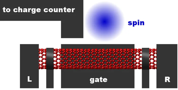
The set-up for our proposed spin meter is shown schematically in figure 1. Any stationary spin can in principle be measured; the details of the physical implementation are not important. For example, it might be a defect spin in a crystal [7], be confined in a semiconductor by a pattern of lithographic electrodes [8] or be a molecular spin [9]. A general obstacle to the sort of device we are proposing is the wide range of relevant energy scales, which at first seems to preclude sensitive spin measurement. An estimate of the dipole–dipole interaction

2

Figure 1.An implementation of the spin meter concept. The central part of the device is a quantum dot that is defined by electrical gates that pinch off a one-dimensional conductor, such as a nanowire or a carbon nanotube. The electrical transport through the quantum dot can be controlled with high precision by varying the source and drain potentials and the potentials of the extra finger gates placed at the junctions. The charging state of the dot can be sensed through an electrometer charge counter, which is coupled to the quantum dot by a conducting bridge, and a back gate can control the number of electrons on the quantum dot. A single spin is placed close to the quantum dot. If there is no electron hopping between the dot and the spin site, then the main coupling mechanism between the electron spin on the dot and the spin we want to read out is the dipole–dipole interaction. In such a set-up no current will flow directly through the region where the spin is located and thus the spin will not be disturbed.

energy between two electron spins is J _≈100r₀3/r3MHz, where r0=1 nm. For a successful

measurement, the current flow through the dot has to be sensitive to the corresponding energy change. The energy resolution of the dot is usually governed by the width of a typical electronic energy level, which depends on the tunnelling rate and, more importantly, by the temperature-dependent width of the Fermi function for the electrons in the leads. With attainable temperatures in standard dilution refrigerators (∼10 mK) the energy resolution of the dot becomes∼1 GHz, clearly not enough to resolve the dipole–dipole interaction.

This obstacle can be overcome by considering spin resonance effects that are introduced by applying microwave radiation. Recently, there has been increasing interest in methods for electrical detection of spin resonance [10, 11]. Mozyrksy et al [12] showed that the current in a quantum channel next to an impurity spin depends on the frequency of the incident microwave. We recently showed that a similar resonant change in the current takes place in transport through a quantum dot [13]. The line width of the resonance introduces a new energy scale into the energy dependence of the dot occupations that can be much smaller than the temperature, subsequently enabling the detection of much smaller shifts in energy. Typical microwave intensities correspond to frequencies of∼1 MHz but can be made smaller, provided that the lifetime of the electron on the dot is sufficient to allow for equalization of the spin

Rabi frequency. Given a controllable tunnelling rate the sensitivity of the dot detector can be increased by lowering the microwave intensity and also the tunnelling rate, with the lower limit set by the coherence time of the spin on the dot.

The simplest model capturing all the relevant physics consists of two spin-1/2 particles, one situated on the quantum dot (the flying spin) and the other nearby (the stationary spin). In a magnetic field, the energy levels for spin up and spin down for each of the spins will be split by the Zeeman energy, but in general the splitting will be different for the flying and the stationary spin whoseg-factors are typically unequal. Thus any incident narrow-band microwave radiation can only be resonant with one of the spins. We choose it to be resonant or nearly resonant with the flying spin. The dipole–dipole and exchange coupling between the two spins give rise to an effective Ising interaction, since flip–flop processes are suppressed by the Zeeman terms. The resulting Hamiltonian in the rotating frame after the rotating wave approximation can be written as

H ₌ 10S 2 σ

(S)

z +

10F

2 σ (F)

z +



2σ (F)

x +

J

2σ (S)

z σ(

F)

z ,

where S labels the stationary spin and F the flying spin, and 10S/F=gS/FµBBz− ¯hω0, with

Bz being the magnetic field in the z-direction, µB the Bohr magneton, gS/F the g-factor for

the stationary/flying spin, respectively, and ω0 the microwave frequency. The Rabi frequency

due to an oscillating magnetic field in the x-direction for the flying spin is; we can neglect the equivalent term for the off-resonant static spin. J is the Ising interaction strength. The Hamiltonian separates into two decoupled subspaces, associated with stationary spin up (↑) and spin down (↓), respectively, and is written as follows:

H_↑/↓= 1

210↑/↓σ (F)

z +



2σ (F)

x ∓

10S

2 ,

where we defined the spin subspace-dependent detuning 10↑/↓=10F∓J. The upper/lower

sign refers to the up/down subspace.

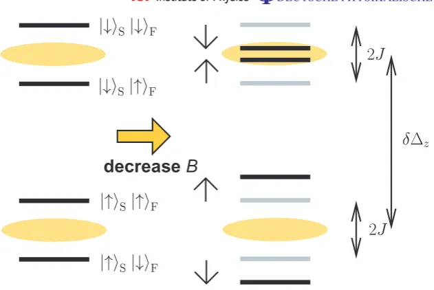
The resulting energy level structure is shown in figure 2. Decreasing the magnetic field will shift the upper pair of levels towards resonance, with the Rabi frequency dominating their splitting. Meanwhile, the splitting of the lower pair increases. Close to resonance the eigenstates become products of the static spin state with linear superpositions of flying spin up and flying spin down:

|aiF =as↑|↑iF+as↓|↓iF,

|biF =bs↑|↑iF+bs↓|↓iF,

s_=↑, _↓denotes the stationary spin subspace. The detuning-dependent coefficients are given by

as↑/↓=

v u u u t 1 2 

1±

10s q

12 0s+2



,

wherebs↑= −as↓ andbs↓=as↑.

4

decrease

B

δΔz

|↑_S|↑_F |↓_S|↑_F

2J

2J |↓_S|↓_F

|↑_S|↓_F

Figure 2. The level structure of the two-spin system in the rotating frame for

10F=0. After decreasing the magnetic field the upper two levels (stationary spin

down subspace) move into resonance. The difference in the Zeeman splittings is given byδ1z=10S−10F.

Quantum dot

γ>

R↓

γ<

R↑ γ>

R↑ γ>

L↑

γ<

L↑ γ>

L↓ γ<

L↓

|b_F

|a_{F γ}<

R↓

Right lead Left lead

Figure 3. A schematic diagram showing tunnelling off and onto the quantum dot. The states on the quantum dot are superpositions of spin up and spin down. The rates for tunnelling on and off the quantum dot depend on the spin, the bias voltage, temperature, Zeeman splitting and gate voltage.

the spin down subspace), we can analyse the rates of tunnelling from the leads onto the dot and from the dot into the leads. The tunnelling can be studied in detail using a master equation approach [13]. For the populations, the master equation results can be presented as simple rate equations. A schematic depiction of the tunnelling rates is shown in figure3.

To derive the rate equations, let us consider the stationary spin up subspace and concentrate on the change in population of the state |a_iF. For the population to increase the dot has to be

energy for state|a_iF. The lead electron can come either from the left or the right lead and can have either spin up or spin down. Considering the tunnelling rate for spin up electrons in the left lead onto the state| ↑iF, we get the tunnelling rate

γ<

L↑=γ0f(µL− ¯hω0/2),

where now f()₌1/(1 + exp(β))is the Fermi function and gives the probability of finding an occupied electron state with spin up in the left lead. The maximum tunnelling rate is given by

γ0. Since the state|aiFhas spin up and spin down components the rate has to be reduced by the

probability that _|a_iF is in state_|↑iF, i.e. by a factor _|a_↑↑|2_{. Similarly, we can deduce the rates}

for spin down and also for the right lead. For the population in state|a_iFto decrease, state|a_iF has to be occupied, with probability p_↑a and an empty state at the corresponding energy in one

of the leads and spin subspaces has to be found. Considering again the tunnelling rate from the state|↑iFto spin up electrons in the left lead, we get the rate

γ>

L↑=γ0[1− f(µL− ¯hω0/2)],

where now the probability of finding an empty state at energyis given by 1− f(). Only part of the state|a_iFis in state|↑iF, and therefore we have to reduce the rate again by|a_↑↑|2. Taking every possible tunnelling process into account, we arrive at the rate equations for the stationary spin up subspace, as

˙

p_↑a = |a↑↓|2γ↓<+|a↑↑|2γ↑<

p_↑0− |a↑↓|2γ↓>+|a↑↑|2γ↑>

p_↑a, (1)

where p_↑a is the probability of finding the stationary spin in state↑and the flying spin in state

|a_iF and p_↑0 is the probability of finding the stationary spin in state ↑ and no electron on the dot,γ_↑<_/↓are the tunnelling rates onto the dot from either spin up or spin down states in the leads andγ_↑>_/↓are the tunnelling rates off the dot for different spin populations. They are given by

γ<

↑/↓=γL<↑/↓+γR<↑/↓, γ↑>/↓ =γL>↑/↓+γR>↑/↓

where the tunnelling rates from the left and right leads are given by

γ<

L↑=γ0f(µL− ¯hω0/2), γL>↑ =γ0[1− f(µL− ¯hω0/2)] γ<

L↓=γ0f(µL+h¯ω0/2), γL>↓=γ0[1− f(µL+h¯ω0/2)],

with similar equations for the right lead. f()₌1/(1 + exp(β))is the Fermi function and the chemical potentials in the left and right leads are given byµL/R=µ−Vg±Vsd/2 withµbeing

the chemical potential without voltage bias, Vg the gate voltage and Vsd the bias voltage. A

similar rate equation holds for the population of the other energy eigenstate

˙

p_↑b= |b↑↓|2γ↓<+|b↑↑|2γ↑<

p_{↑0− |}b_↑↓|2γ_↓>+|b_↑↑|2γ_↑>p_↑b. (2)

Additionally, the individual probabilities have to add up to the probability of finding the stationary spin in a spin up state p_↑= p_↑a+p↑b+ p↑0. The equivalent rate equations can be

derived for the stationary spin down subspace and p_↑+p_↓=1. The stationary state can be obtained for each stationary spin subspace from ˙p_↑a/b/0=0 and ˙p↓a/b/0=0 and we obtain

the average population on the quantum dot as a function of the applied magnetic field,

6

n

Δ

0

Δn αΩ

−J J

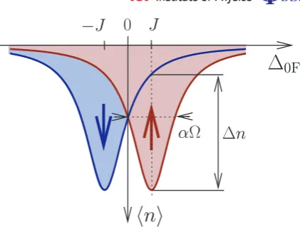
Figure 4.The average dot populationhn_ias a function of the detuning10F for

stationary spin up and spin down, respectively. The two Lorentzian peaks are centred at_±J and have a width ofα. Observing the population at a detuning of +J the difference in population between the case where the stationary spin points up and where the stationary spin points down is given by1n.

with

L(1)₌ 1

2_r

∞+2r0

12₊α22 . (4)

The coefficients in the Lorentzian equation (4) are given by

r_∞= (1− f+)

2 − f₋2 1 + f₋2₋ f2

+

, r₀₌ (1− f+)

2

1 + f₋2₋ f2 + ,

and

α2

= 1− f 2 +

1 + f₋2₋ f2 +

with f+= 1₂

f_↑L+ f↑R+ f↓L+ f↓R

, f₋₌ 1₂f_↑L+ f↑R− f↓L− f↓R

and f_↑/↓x = f(µx∓ ¯hω0),

wherex ₌L,R.

The behaviour of the average dot population, equation (3), as a function of the detuning is shown in figure 4. If we want to distinguish spin up from spin down we can monitor the population at resonance, say 10F=J. The change in population from a pure spin up state

(p_↑=1) to a pure spin down state (p_↓=1) is given by

1n₌L(0)−L(2J).

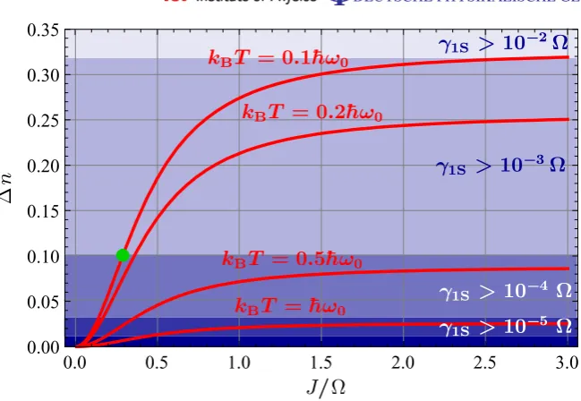
The dependence of 1n on the spin–spin interaction strength J and the temperature is shown in figure5. The change in occupation number decreases with an increase in temperature and a decrease in spin–spin interaction strength. In order to detect a small change in the dot occupation number, a certain number of electron tunnelling events have to take place. To detect a change of1n, more than 1/1n2electrons have to tunnel; therefore the electron tunnelling rate needs to be much larger than the stationary spin relaxation time. In order to see a resonance of the spin on the quantum dot, two things have to be fulfilled: the Rabi frequency has to be stronger

0.0 0.5 1.0 1.5 2.0 2.5 3.0 0.00

0.05 0.10 0.15 0.20 0.25 0.30

kBT = 0.2¯hω0

γ1S > 10−3_Ω

γ1S > 10−4 Ω γ1S > 10−5 Ω

J/Ω

∆

n

kBT = 0.1¯hω0

kBT = 0.5¯hω0

kBT = ¯hω0

Figure 5. Change of the charge on the quantum dot between spin up and spin down on the stationary spin as a function of the exchange coupling between the stationary and the flying spin for small bias voltages (V_sd=0.1, V_g=0). Different curves are for different temperatures. The blue shading in the background indicates the detectable change in occupation given a certain relaxation time of the stationary spin. The green dot indicates the example discussed in the text.

than any spin relaxation, intrinsic or tunnelling induced, and the thermal spin polarization has to be significantly different from zero. For a non-demolition measurement the difference in the spin Zeeman splittings between stationary and flying spin has to be much larger than the Rabi frequency and the spin–spin interaction.

How does this translate to experimental parameters? With a spin coherence time of 1µs on the carbon nanotube quantum dot, we need a Rabi frequency of at least=10 MHz to drive the spin into saturation, and thus effect a change of the on dot spin occupation. Given the standard ESR microwave frequency ofω0=10 GHz and the corresponding magnetic field of 350 mT, at

dilution refrigerator temperature (T ₌50 mK) we can read out a spin with a relaxation time of 0.1 ms and a coupling of J ₌3 MHz. Since the electron spin on the quantum dot is delocalized we cannot directly apply the rule of thumb J _≈100r₀3/r3MHz. An estimate of the effective coupling strength can be obtained by assuming a constant particle density on the quantum dot. Assuming that the stationary spin is located at the centre of the quantum dot, the effective coupling becomes

J ₌ J0r

3 0

L

Z L/2

−L/2

dx 1

r2_+x23/2 = J0 _r

0

r

3

2r L,

where J0=100 MHz,r0=1 nm, L is the length of the quantum dot andr is the perpendicular

8

of a molecular magnet spin [14]. Hopping between the spin site and the nanotube does not inhibit the readout as long as the binding energy of the electron at the spin site is sufficiently different from the energy of the conduction electrons of the nanotube. In this case the hopping would only lead to an effective exchange interaction between the electrons on the nanotube and the electron on the spin site in addition to dipolar coupling. Indeed, using a conductive molecule to attach the spin to the nanotube could increase the coupling strength, making reliable readout easier or allowing larger distances between the nanotube and spin.

With the above example we want to highlight a particular case of spin readout that can be achieved with our proposed technology, but the scheme works also in other parameter regimes: given a spin with much longer relaxation times, e.g. N@C60 with aT1 of minutes at 4 K [15],

reliable readout can be achieved at either weaker couplings or a larger thermal energy to Zeeman splitting ratios. Given the same quantum dot parameters as above and a coupling strength of J ₌3 MHz, the readout will work at T ₌4 K and a magnetic field of 600 mT. On the other hand, given the same temperature and magnetic field as above, a spin with a coupling strength of J ₌0.25 MHz can be read out. With only dipole–dipole coupling, this corresponds to a separation of the quantum dot and the spin of≈2 nm.

Quantum dots in nanotubes have been fabricated (see e.g. [16, 17]), also with integrated charge counters [18, 19], and on-chip microwave resonators reaching Rabi frequencies of

∼10 MHz have been demonstrated (e.g. [20, 21]). We therefore conclude that our scheme is realizable with current technology.

Acknowledgments

We thank the QIPIRC (GR/S82176/01) for support. BWL thanks the Royal Society for support through a University Research Fellowship. JW thanks the Wenner-Gren Foundations for financial support. We thank J H Wesenberg and S C Benjamin for discussions.

References

[1] Hanson R and Awschalom D D 2008 Coherent manipulation of single spins in semiconductorsNature453

1043

[2] Maze J Ret al2008 Nanoscale magnetic sensing with an individual electronic spin in diamondNature455

644

[3] Sarovar M, Young K C, Schenkel T and Whaley B K 2008 Quantum nondemolition measurements of single donor spins in semiconductorsPhys. Rev.B78245302

[4] Lu H-Z and Shen S-Q 2008 Using spin bias to manipulate and measure spin in quantum dotsPhys. Rev.B77

235309

[5] Rugar D, Budakian R, Mamin H J and Chui B W 2004 Single spin detection by magnetic resonance force microscopyNature430329

[6] Elzerman J M, Hanson R, Willems van Beveren L H, Witkamp B, Vandersypen L M K and Kouwenhoven L P 2004 Single-shot read-out of an individual electron spin in a quantum dotNature430431

[7] Wrachtrup J and Jelezko F 2006 Processing quantum information in diamondJ. Phys.: Condens. Matter18

807

[8] Hanson R, Kouwenhoven L P, Petta J R, Tarucha S and Vandersypen L M K 2007 Spins in few-electron quantum dotsRev. Mod. Phys.791217

[9] Bogani L and Wernsdorfer W 2008 Molecular spintronics using single-molecule magnetsNat. Mater.7179

P spin quantum statesNat. Phys.2835

[11] Xiao M, Martin I, Yablonovitch E and Jiang H W 2004 Electrical detection of the spin resonance of a single electron in a silicon field-effect transistorNature430435

[12] Martin I, Mozyrsky D and Jiang H W 2003 A scheme for electrical detection of single-electron spin resonance

Phys. Rev. Lett.90018301

[13] Wabnig J, Lovett B W, Jefferson J H and Briggs G A D 2009 Spin lifetimes in quantum dots from noise measurementsPhys. Rev. Lett.102016802

[14] Ardavan A, Rival O, Morton J J L, Blundell S J, Tyryshkin A M, Timco G A and Winpenny R E P 2007 Will spin-relaxation times in molecular magnets permit quantum information processing?Phys. Rev. Lett.98

057201

[15] Morley G W 2005 Designing a quantum computer based on pulsed electron spin resonance PhD Thesis

(Oxford: University of Oxford)

[16] Tans S J, Verschueren A R M and Dekker C 1998 Room-temperature transistor based on a single carbon nanotubeNature39349

[17] Jørgensen H I, Grove-Rasmussen K, Hauptmann J R and Lindelof P E 2006 Single wall carbon nanotube double quantum dotAppl. Phys. Lett.89232113

[18] Biercuk M J, Reilly D J, Buehler T M, Chan V C, Chow J M, Clark R G and Marcus C M 2006 Charge sensing in carbon-nanotube quantum dots on microsecond timescalesPhys. Rev.B73201402

[19] Gotz G, Steele G A, Vos W-J and Kouwenhoven L P 2008 Real time electron tunneling and pulse spectroscopy in carbon nanotube quantum dotsNano Lett.84039–42

[20] Mamin H J, Budakian R and Rugar D 2003 Superconducting microwave resonator for millikelvin magnetic resonance force microscopyRev. Sci. Instrum.742749

[21] Narkowicz R, Suter D and Stonies R 2005 Planar microresonators for EPR experimentsJ. Magn. Res.175