DOI 10.1007/s10651-017-0376-0
Estimation bias under model selection for distance
sampling detection functions
Rocio Prieto Gonzalez1 · Len Thomas1 · Tiago A. Marques1,2
Received: 15 October 2016 / Revised: 1 May 2017
© The Author(s) 2017. This article is an open access publication
Abstract Many simulation studies have examined the properties of distance sampling estimators of wildlife population size. When assumptions hold, if distances are gener-ated from a detection model and fitted using the same model, they are known to perform well. However, in practice, the true model is unknown. Therefore, standard practice includes model selection, typically using model comparison tools like Akaike Infor-mation Criterion. Here we examine the performance of standard distance sampling estimators under model selection. We compare line and point transect estimators with distances simulated from two detection functions, hazard-rate and exponential power series (EPS), over a range of sample sizes. To mimic the real-world context where the true model may not be part of the candidate set, EPS models were not included as can-didates, except for the half-normal parameterization. We found median bias depended on sample size (being asymptotically unbiased) and on the form of the true detection
Handling Editor: Pierre Dutilleul.
Electronic supplementary material The online version of this article (doi:10.1007/s10651-017-0376-0) contains supplementary material, which is available to authorized users.
B
Rocio Prieto Gonzalez [email protected] Len Thomas[email protected] Tiago A. Marques
1 CREEM, University of St Andrews, The Observatory, Buchanan Gardens, St Andrews KY16 9LZ, UK
function: negative bias (up to 15% for line transects and 30% for point transects) when the shoulder of maximum detectability was narrow, and positive bias (up to 10% for line transects and 15% for point transects) when it was wide. Generating unbiased simulations requires careful choice of detection function or very large datasets. Prac-titioners should collect data that result in detection functions with a shoulder similar to a half-normal and use the monotonicity constraint. Narrow-shouldered detection functions can be avoided through good field procedures and those with wide shoulder are unlikely to occur, due to heterogeneity in detectability.
Keywords Detection models·Line transect·Model selection·Point transect· Wildlife abundance estimation
1 Introduction
Distance sampling (DS,Thomas et al. 2002;Buckland et al. 2001,2015) is used widely
for estimating the size and spatial density of wild animal populations. It includes two main methods, line transect sampling (LTS) and point transect sampling (PTS). In both, the observer performs a survey along a randomly located series of lines (LTS) or points (PTS) and measures distances to detected animals. Not all animals in the vicinity of transects will be detected: typically the proportion of animals detected decreases with
increasing distance from the transect. A key concept is the detection functiong(y),
which models the probability of detecting an animal, given its distance y from the
transect. DS analysis uses Horvitz–Thompson-like estimators, since the probability of
detection is unknown, and must be estimated (Borchers 1996;Buckland et al. 2001).
This is achieved by fitting a model for the detection function to the observed distances. DS is therefore a composite approach, as it cannot be considered entirely design-based
(Fewster and Buckland 2004;Barabesi and Fattorini 2013), being dependent on a good
model forg.
The method relies on 4 assumptions (Buckland et al. 2001, pp. 29–37):
1. Transects are located at random, ensuring that animals are distributed indepen-dently of the transects. This ensures the true distribution of animals with respect to the line or point is known (being uniform or triangular, respectively).
2. The probability of detecting an animal on the transect or point is 1,g(0)=1.
3. Distances are measured without errors.
4. The survey can be seen as a snapshot in time, during which animals do not move.
DS estimators are asymptotically unbiased when assumptions are met (Buckland
et al. 2015, p. 117). In simulations where assumptions hold and distances are generated
from a particular model and fitted using the same model, methods seem to perform
well (e.g.Buckland 2006;Du Fresne et al. 2006;Glennie et al. 2015). However, in
real life situations, we face two additional issues not typically accounted for in pre-vious simulation studies. First, the true detection function is unknown. Therefore, the
standard methods for fitting detection functions to DS data, as described byBuckland
et al.(2001), and which we refer to collectively as “conventional distance sampling”,
involve selecting among several classes of flexible, semi-parametric models.Buckland
using standard model selection techniques such as choosing the model with mini-mum Akaike Information Criterion (AIC). Second, for a reliable estimate, we need to
achieve an adequate number of detections:Buckland et al.(2001) recommend at least
60–80 for lines and 75–100 for points. Despite the usual recommendation, reported
sample sizes very often do not reach these values (e.g.Buckland 2006;Williams and
Thomas 2007;Durant et al. 2011).
This study was motivated by finding non-negligible bias in DS estimators, in a simulation scenario involving moderate sample size and model selection, as part of a larger study looking at violation of the no movement assumption. Before animals started moving (thus the assumptions were met) no bias was expected, but was clearly present. Rather than fitting from the true model, we were using model selection, and soon it became apparent that this was the source of the bias. This lead us to question the sample size guidelines, and also the effect of the shape of the true detection function model, and hence undertake the study reported here.
Many simulations studies have considered AIC for detection model selection (e.g.
Cassey and Mcardle 1999;Ekblom 2010;Borchers et al. 2010) but their main interest
was the robustness of DS estimators and their asymptotic properties, so large sample sizes were used. Moreover, the distances came from a particular shape of one detection
function. One exception to this isMiller and Thomas(2015), who fit mixture models to
a variety of DS detection functions and sample sizes. In some of the more challenging and potentially problematic scenarios considered, they found median biased estimators (an estimate is median-unbiased if it underestimates just as often as it overestimates) of average detection probability (they did not report bias in estimated abundance), even when the sample size was large. At small sample sizes, median biased estimates were found even in some standard cases, although they did not make a comprehensive assessment. We have not found any simulation studies that consider the combination of a wide variety of true detection function shapes and range of sample sizes (low, mod-erate and large) using detection model selection, hence the novel aspect of this study. Here, we evaluate by simulation the performance of DS estimators when assump-tions 1–4 hold and the model adopted for fitting the detected distances is selected from a set of candidate models, differentiating two cases: (1) including or (2) exclud-ing the true detection function from the set of candidate models. We also test whether the existing sample size recommendations are reliable, and compare LTS and PTS estimators over a range of detection function shapes.
The remaining sections are organized as follows. In Sect.2we describe the
simula-tion scenarios and analysis performed on simulated data. We present the main results
in Sect.3, while many additional results are given in online supplementary materials.
Finally, in Sect.4, we discuss the implications of our study for both simulation studies
and real-world DS surveys.
2 Methods
2.1 Conventional distance sampling
Let N be the abundance (i.e., population size) of animals in a study area of size
A, and let D = NA be the animal density. N is estimated by Nˆ = ˆn
PaaA, wheren
is the number of detected animals in the surveyed areaa, and Pˆa is the estimated
average probability of detecting an animal withina. The density estimator is obtained
simply by dividing the abundance estimator by A, Dˆ = ˆn
Paa. Discarding any
obser-vations beyond a truncation distancew, the sampled areaais 2Lwfor line transects
of total line length L, andkπw2forkpoint transects. Estimated density for LTS is
ˆ
D=n2fˆL(0), where fˆ(0)is the value of the pdf of detected distances evaluated at zero
distance (Buckland et al. 2001, pp. 38–41). For LTS, f(y)andg(y)have identical
shape, only rescaled so that f integrates to unity, because the area of a strip of
incre-mental widthd yat distanceyfrom the line is independent ofy. For PTS,Dˆ = n2fˆπ(k0)
with fˆ(0)being the derivative of the pdf evaluated at zero. The area of a ring of
incremental widthd yat distanceyfrom the point is proportional toy, thus f(y)is
pro-portional toyg(y). These two estimator expressions make it explicit that the behaviour
of the pdf at zero distance is critical for estimating animal density for both points and lines.
2.2 Data simulation
The simulation was conducted using R software (R Core Team 2014, version 3.2.4).
For each simulated dataset, detection function estimation (see Sect.2.3) was performed
using the MCDS engine from the software Distance (Thomas et al. 2010, version 6.2),
except for the EPS true model, not available in Distance and hence coded in R. The simulation code is available in Online Resource 1 (hereafter OR1).
The focus of our simulation was on the potential relative bias caused by detection function estimation. Hence, we used a very simple study area, animal distribution and spatial sampling scenario. Our results on bias will not be sensitive to these choices, so long as random sampling is used; however, those relating to variance and confidence interval estimation will be. The study area considered for simulation was a square of
area A =1 km2. For each simulation iteration, a fixed number,N, of animals were
located at random according to a uniform density distribution within the study area. A fixed number of transects were laid at random locations within the area. For LTS, lines were oriented perpendicular to the x-axis, making them 1 km long. For both LTS
and PTS a truncation distance ofw=30 m was used. We used 5 lines and 106 points,
making the surveyed areaa =0.30 km2in both cases.
For each animal within the truncation distancewof a line or point, we calculated its
distance,y, to the line or point. According to a given detection functiong, a random
draw from a Bernoulli distribution withp=g(y)determined whether it was detected
or not.
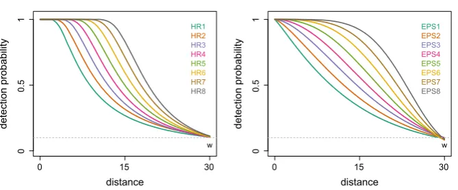
The detections were generated from 8 different parameterizations of 2 detection
functions, with 2 parameters each (Fig.1): the hazard-rate (HR) and the exponential
distance
00
.5
1
detection probability
w HR1
HR2 HR3 HR4 HR5 HR6 HR7 HR8
distance
0 15 30 0 15 30
00
.5
1
detection probability
w EPS1
EPS2 EPS3 EPS4 EPS5 EPS6 EPS7 EPS8
Fig. 1 Different parametrizations of the true detection function to generate the observed distances. On the
lefta hazard-rate (HR) and on therightan exponential power series (EPS). Thedashed lineisg(w)=0.1
hazard-rate:g(y;σ,b) =1−exp
−y
σ −b
σ >0; b>0
EPS: g(y;λ, α)=exp
−y
λ α
λ >0; α >0
(1)
Whenα=2 (EPS4), the EPS corresponds to the standard half normal (HN)
distribu-tion, frequently used in DS analysis.
Parameters of the true detection function were chosen such thatg(w)=0.1, in line
with the recommendation fromBuckland et al.(2001) that right truncation occur when
g(w)≈0.1. The parameter values used are shown in OR1, Table 1. They were chosen
so that the resulting detection functions had a variety of shapes. In mathematical terms, the shoulder of the detection function is the range of distances from the line or point for
which the slope (g) is zero; in other words, the range of distances which probability of
detecting an animal is one. Thus, the shape of the detection functions considered goes from having no shoulder (also known as spiked data) to having a wide flat shoulder
(c.f. Fig.1).
For each scenario, the true population size,N, was chosen to give a pre-determined
expected sample size of observations, E(n). For each true detection function, we
ran simulations withE(n)= {60,90,120,240,500,5000}(see OR1, Table 2). For
each scenario we simulated 4000 iterations, to reduce the relative Monte Carlo error
associated with the standard error of the N estimator (calculated using Equation (7)
inKoehler et al. 2009) to below 1%.
2.3 Analysis of simulated data
For each of the simulated datasets, we fitted all the model combinations recommended
byBuckland et al.(2001). In that framework, the detection function has two parts, a key
function and a series expansion:g(y)∝key(y)[1+series(y)]. The series expansion
is used to provide additional flexibility to fit the data, if required. Each parametric
key function was paired with the suggested series adjustment term given byBuckland
[image:5.439.55.390.48.187.2]Table 1 Detection function models fitted to the simulated data
Key function Series expansion Uniform,w1 Cosine,Σmj=1ajcos
jπy w
Uniform,w1 Simple polynomial,
Σm j=1aj
y w2j
Half-normal,ex p
−y2
2σ2
Cosine,Σmj=2ajcos jπy
w
Half-normal,ex p
−y2
2σ2
Hermite polynomial,
Σm
j=2ajH2j(ys)where
ys= σy
Hazard-rate, 1−ex p
−y σ−b
Cosine,Σmj=2ajcos jπy
w
Hazard-rate,
1−ex p−σy−b
Simple polynomial,
Σm
j=2ajwy2j
g(y)∝key(y)[1+series(y)], whereyis the distance from the transect to the target object,w the truncation distance, andσ andbthe scale and shape parameter respectively;mis the maximum number of terms in the series expansion,
aj∈R∀j=1, . . . ,mis the
parameter of termj
As is standard in the Distance software, we selected the number and order of adjustment terms required for the analysis using sequential forward selection, starting with no adjustments, and adding one at a time, so long as the resulting model had a lower AIC than the previous one. We considered at most 5 parameters for the detection function, the default in the Distance software. When adjustments are selected, the detection function can be non monotonic. The default in Distance, to constrain the fitted functions to be monotonically non-increasing (i.e., either flat or decreasing), was also considered. This is referred to as simulation scenario 1.
A potential source of bias when the true detection function has a wide shoulder is model selection being too conservative or/and the monotonicity constraint. Con-sequently, we investigated further by running five additional simulation scenarios. First (scenario 2.1), we relaxed the monotonicity constraints on the detection func-tion, allowing the curve to take any possible form, constrained to be non-negative. Second, besides turning off the monotonicity constraint, we also set the number of parameters to be the same in all the candidate models. This lead us to select the model that fits the best when the parameter penalty was the same for all of them. Because the true models both have two parameters, we restrained the number of parameters first to two (scenario 2.2) and then three (scenario 2.3), being the goal of the three parameter model constraint to test whether the 2-parameter detection function was flexible enough. This implies 0 or 1 adjustment terms for HR, 1 or 2 for HN, and 2 or 3 for uniform keys, respectively for Scenarios 2.2 and 2.3. Finally, we constrained the number of parameters to two (scenario 2.4) and three (scenario 2.5) without the monotonicity constraint being lifted.
to be selected, whereas the EPS distribution, not being available in Distance, was never included in the candidate set (except for the special case of the half normal
parametrization,α=2). As a consequence, we could not use Distance software to fit
the EPS under the true model scenarios, and a bespoke likelihood and the R function “optim” was used instead. The few cases where the algorithm did not converge were discarded.
As noted above, we simulated from detection functions with parameters chosen such
that true detection probability at the truncation distance,g(30), was approximately 0.1.
Because more truncation tends to reduce the bias when we select the wrong model, we investigated the effect that truncating the data at the analysis stage has on bias, just
for the average sample size of 240 case, by using a truncation distance ofw=20.
2.4 Processing of results
The median percentage bias in Nˆ was estimated for the 4000 replicates of each
sce-nario: for each set of parameters of the HR and EPS true model, in both LTS and PTS scenarios and for each mean sample size. We calculated both the bias produced by the selected detection function, under model selection (i.e., the function with lowest AIC for each replicate dataset) and by the fitted true detection function. Instead of more commonly used mean bias, we considered median bias to reduce the influence of some
very large overestimates ofN that occasionally occurred. The mean percentage bias
is given in OR1. We also show percentage bias inPˆain OR1, for comparability with
Miller and Thomas(2015). For plotting purposes, the percentage bias was represented
as smooth lines across the eight parametrizations of the true model, to show the pattern with increasing sample size.
Estimator performance was also evaluated by the percentage relative root mean square error (RRMSE), which measures the overall variability, incorporating the vari-ance of the estimator and its bias.
The 95% confidence intervals on average probability of detection were estimated
for each iteration. We considered Nˆ to be log-normally distributed, as described in
Buckland et al. (2001, Section 3.6.1).
In OR1, we also present coverage probabilities (proportion of intervals containing
the true value) for confidence intervals forN.
3 Results
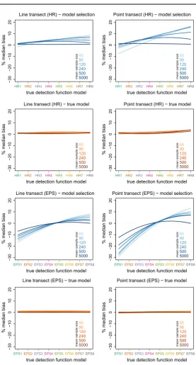
As expected, abundance estimators were close to median-unbiased when the true model was fitted, and bias decreased with increasing sample size. By contrast, under model selection, there was a consistent pattern in median bias: bias was negative for data generated from detection functions with a small shoulder and positive for those
with a wide shoulder (Fig.2; raw results are given in OR1 Figs. 1–4). The pattern
was stronger for points than lines, and for smaller sample sizes. For the HR model,
median bias atE(n)=60 ranged from−3 to+8% for LTS and−8 to+15% for PTS.
Results were worse for the EPS model, where the true model was not in the candidate
true detection function model −30 − 20 −10 0 10 20
Line transect (HR) − model selection
% median bias
60 90 120 240 500 5000
mean sample siz
e
HR1 HR2 HR3 HR4 HR5 HR6 HR7 HR8
true detection function model
−30 − 20 −10 0 10 20
Point transect (HR) − model selection
% median bias
60 90 120 240 500 5000
mean sample siz
e
HR1 HR2 HR3 HR4 HR5 HR6 HR7 HR8
true detection function model
−30 − 20 −10 0 10 20
Line transect (HR) − true model
% median bias
60 90 120 240 500 5000
mean sample siz
e
HR1 HR2 HR3 HR4 HR5 HR6 HR7 HR8
true detection function model
−30 − 20 −10 0 10 20
Point transect (HR) − true model
% median bias
60 90 120 240 500 5000
mean sample siz
e
HR1 HR2 HR3 HR4 HR5 HR6 HR7 HR8
true detection function model
−30 − 20 −10 0 10 20
Line transect (EPS) − model selection
% median bias
60 90 120 240 500 5000
mean sample siz
e
EPS1EPS2EPS3EPS4EPS5EPS6EPS7EPS8
true detection function model
−30 − 20 −10 0 10 20
Point transect (EPS) − model selection
% median bias
60 90 120 240 500 5000
mean sample siz
e
EPS1EPS2EPS3EPS4EPS5EPS6EPS7EPS8
true detection function model
−30 − 20 −10 0 10 20
Line transect (EPS) − true model
% median bias
60 90 120 240 500 5000
mean sample siz
e
EPS1EPS2EPS3EPS4EPS5EPS6EPS7EPS8
true detection function model
−30 − 20 −10 0 10 20
Point transect (EPS) − true model
% median bias
60 90 120 240 500 5000
mean sample siz
e
EPS1EPS2EPS3EPS4EPS5EPS6EPS7EPS8
[image:8.439.80.358.40.556.2]for PTS. Median bias inPˆafollowed the opposite pattern to median bias inNˆ (OR1,
Tables 5–6), as would be expected given thatNˆ =n/Pˆa.
Estimators generally showed positive mean bias inNˆ at low and moderate sample
sizes (OR1 Figs. 5–8). When the true model was fitted, this bias was generally small (at least for LTS), and decreased as sample size increased, so that it was effectively
zero for E(n)=5000. Estimators ofPa were close to mean unbiased when the true
model was fitted, even at small sample sizes; however, unbiased estimators for Pa
will be positively biased for N =n/Pa, because symmetric errors about Palead to
right-skewed errors about 1/Pa. This explains the positive mean bias inNˆ observed.
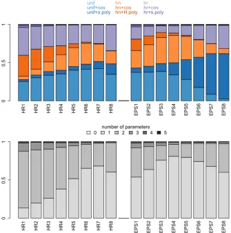
To better understand the median bias pattern under model selection as the shoulder width of the detection function changes, we examined the percentage of times each type of key function + adjustment model was selected, and also the proportion of times
a model withkparameters, wherek∈ {0,1, . . . ,5}, was chosen (OR1 Figs. 10–11).
Given similar patterns across sample sizes and LTS versus PTS, we focus here on an average sample size of 120 observations, which should be adequate for good model
selection (Fig.3). More than half of the time (except for HR1–4) a 1-parameter model
was selected: either unif + cos (Fourier series), unif + simple polynomial expansion, both with only one adjustment term, or HN with no adjustments. HR was not selected often, even when HR was the true model. In this situation it was selected slightly more when the detection function was spiked or flat. One parameter models took over increasingly as the shoulder of HR detection function widened (e.g., HN takes over HN + cos). When EPS was the true model, unif + simple polynomial expansion seemed to take over from unif + cos with the wider shoulder. When data were generated by an HN (EPS4) function, and hence the true model was included in the set of candidates for model selection, despite the true function not being selected most often, the estimator was nearly median-unbiased. Thus AIC seemed useful for selecting the best model
for predictingPain the set, which was not always the true model.
Further, to understand how different models being selected influence bias, we exam-ined the relationship between the selected model and distribution of observed errors (i.e., difference between estimates and true value). We focus here on the worst sce-nario in terms of bias for the selected 120 average sample size, i.e., EPS under PTS
(Fig.4); results for the other scenarios were similar but less extreme (OR1 Figs. 12–
15). For parametrizations with narrow shoulders (EPS1–4) most of the selected models
tended to underestimateN. From EPS4 onwards, estimators were unbiased for almost
all selected models, until those parametrizations with a flat wide detection function
shoulder (EPS7–8) where almost all of the models overestimatedNon overage. This
pattern was consistent for all the selected models except for the HR, which seems to be the only model in the candidate set of models with the opposite pattern: from positive to negative error with increasing shoulder width. However even when the HR was the true model, 1 parameter models were more often selected. Outlier sample estimates, with the largest absolute errors, seemed to be associated with the HR + adjustment term models. The number of outliers decreased when sample size increased. When the true model was fitted, the percentage error was smaller (OR1 Figs. 16–19).
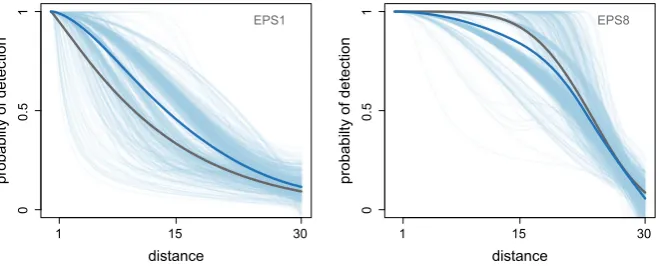
Examining the selected detection functions (Fig.5), we see that when the true
unif unif+cos unif+s.poly
hn hn+cos hn+H.poly
hr hr+cos hr+s.poly
HR1 HR2 HR3 HR4 HR5 HR6 HR7 HR8 EPS1 EPS2 EPS3 EPS4 EPS5 EPS6 EPS7 EPS8
00
.5
1
00
.5
1
number of parameters
0 1 2 3 4 5
HR1 HR2 HR3 HR4 HR5 HR6 HR7 HR8 EPS1 EPS2 EPS3 EPS4 EPS5 EPS6 EPS7 EPS8
Fig. 3 Proportion of time each candidate model class (above) and each model with a fix number of parametersk∈ {0,1, . . . ,5}(below) is selected in a point transect scenario for the 8 sets of parameters of the hazard-rate (HR) and exponential power series (EPS) distributions, with an expected sample size of 240 observations
on average to be flatter than the true detection function. This resulted in overestimation
of Paand hence underestimation ofN. Conversely, when the true detection function
had a wide shoulder (e.g., EPS8), the selected functions tended on average to have
a more rounded shoulder and hence underestimated Paand overestimated N. These
patterns are intuitively sensible once we overlay a representative fitted detection
func-tion to the data it is being fitted to. When we had spiked data (e.g., Fig.6), we tended
to have models that cut the spike of the observed distance distribution (having a lower
intercept), resulting in overestimating Pˆa, and therefore underestimatingNˆ. By
con-trast as the shoulder of the detection function widened, the opposite happens.Pˆawas
[image:10.439.52.388.56.395.2]true detection function model
EPS1 EPS2 EPS3 EPS4 EPS5 EPS6 EPS7 EPS8
−50
100
200
3
00
% error
unif unif+cos unif+s.poly
hn
hn+cos hn+H.poly
hr
hr+cos
hr+s.poly
Fig. 4 Percentage error introduced by each model of the candidate set of model selection detection function, for the 8 sets of parameters of the exponential power series (EPS) distribution under point transect sampling, withE(n)=120.Box plotswidth is proportional to the number of times each model is selected
distance
1 15 30
00
.5
1
probabilty of detection
EPS1
distance
1 15 30
00
.5
1
probabilty of detection
EPS8
Fig. 5 Set of detection functions fitted using detection function model selection (inblue lines) with the average detection function represented by thethick blue line, when the data are generated by the EPS1 and EPS8 distribution (grey line) in a point transect sampling with an expected sample size of 240 observations
When the monotonicity constraint is removed (scenario 2.1), the percentage was lower than that of a monotonically decreasing detection function (OR1 Fig. 22). More-over, fixing the number of parameters to either two or three respectively (scenarios 2.2 and 2.3), the median bias was even more reduced (OR1 Figs. 23–24). This resulted in nearly median unbiased estimators for a wide shoulder. However, we obtained similar results when the number of parameters was constrained to either two or three while retaining the monotonicity constraint (scenarios 2.4 and 2.5), (OR1 Figs. 25–26).
The results presented above had a Monte Carlo Error<1% in the vast majority of
cases, with a maximum of 4% (OR1 Fig. 27).
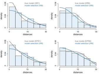
[image:11.439.54.389.51.200.2] [image:11.439.57.387.248.381.2]true model (HR1) model selection (HN)
0 15 30
0
0
.04
0
.08
density
distances
true model (HR8) model selection (HN)
0 15 30
0
0
.04
0
.08
density
distances
true model (EPS1) model selection (HN)
0 15 30
0
0
.04
0
.08
density
distances
true model (EPS8) model selection (HN)
0 15 30
0
0
.04
0
.08
density
distances
Fig. 6 Examples of a particular set of line transect observations (E(n)=120) generated by the first and last parametrization of a HR and EPS distribution (grey line) for which an HN model was selected via model selection (blue line)
Confidence interval coverage was close to the nominal value when the true model was used, and always lower under model selection (OR1 Fig. 29). Under model selec-tion, for HR there appeared to be no particular pattern with width of the shoulder, and in general (but not always), coverage was closer to the nominal level of 0.95 with a large sample size. However, for EPS, coverage appeared to be worse for both spiked data and for wide shoulders, and coverage was low even with large sample size (e.g.,
around 50% for ESP1 and ESP8 withE(n)=500).
Reducing the truncation distance tow = 20 did not help with model selection.
Simulations showed no significant improvement in the problematic cases (see OR1, Fig. 30).
4 Discussion
When a realistic (for most studies) sample size (i.e.,<240) is considered, we found the
bias under model selection depends on several factors: the shape of the true detection function, the use of monotonicity constraints and the number of parameters of the models in the candidate set used for model selection.
First, the median bias inNˆ varies according to the shape of the detection function.
[image:12.439.53.391.50.304.2]selected model, in the majority of cases, bias moves from negative to positive with
increasing shoulder width (Fig. 4, OR1 Figs. 12–15). An exception is the HR and
HR+adjustments, which show the opposite trend. However those models require 2 or more parameters and so are not always selected using AIC; often a 1-parameter model is selected instead. Therefore, the average selected detection function has a
more rounded shoulder than the true model. This leads to an overestimation of P
(underestimation ofN) for more spiked detection functions and underestimation ofP
(overestimation ofN) for detection functions with wider shoulders.
The second factor affecting the bias is the use of the monotonicity constraint in conjunction with the number of parameters of the selected models. The monotonicity constraint is used because we expect a priori that the true detection function is a monotonic non-increasing function of distance from the point or line. However, a particular simulated dataset may be best fit with a non-monotonic function, when by chance there is a small “bump” (cluster of detections) at some distance away from the line. When removing the monotonicity constraint and fixing the number of parameters to be greater or equal than 2, these “bumps” get fitted. This extra flexibility results in a reduction of bias. However, we generally prefer to keep the monotonicity constraint as it is consistent with the process being modelled. We found that keeping this constraint, while fixing the number of parameters to 2, led to a similar reduction in bias. This may be a good strategy for problematic data, particularly PTS where there are relatively few observations close to zero distance.
Bias should not be the only criterion for evaluating estimator performance, as we want estimates with a good balance between accuracy and precision. Yet biased simu-lation scenarios also resulted in greater overall variability when the detection function has a narrow shoulder. We also observed more variability when the true model was fitted and when the sample size was low. The RRMSE for the EPS true model was slightly higher than when model selection is used. This may be due to the optimization routine. When EPS true model is used, fitting occurs in R and we found that the CDS engine in Distance was more robust than optim, the R function we used for
optimiza-tion. In 17 cases out of 4000 iterations (0.425%) a Paestimate lower than 0.04 was
found, giving high values ofN(see OR1, Fitting issues section).
Confidence interval coverage was close to the nominal value when the true model was fitted. Due to the bias found when using model selection over spiked data and wide true detection function shoulders, confidence interval coverage declined to almost 50% in these cases. Our results suggest that when a model selection exercise is conducted,
accounting for model uncertainty should be considered (Burnham et al. 2011). This
should lead to wider intervals and so corresponding improved confidence interval coverage.
Reducing the truncation tow = 20, did not reduce bias under model selection
scenarios. One might think that the more the data are truncated, the less effect the tail
of the detection function has in the estimation of g(0), and hence a more plausible
abundance estimator would be obtained. However, this was not the case here, since no considerable improvement was found in the problematic cases (see OR1, Fig. 27). We did not consider other model selection criteria besides AIC (e.g., AIC with a
correction for finite sample sizes, AICc, or Bayesian Information Criterion, BIC); these
(Burnham et al. 2011) as an alternative. This would make an interesting future study, but it would also be important in this case to consider generating models from true detection functions with more than 2 parameters, to better emulate real-world detection functions.
4.1 Advice on conducting simulation studies
As DS estimators are asymptotically unbiased, with a large enough sample size (i.e., 5000) the bias is negligible. Therefore, when the purpose of the simulation is to evaluate effects of violation of assumptions, without the results being affected by small-sample issues, we recommend using very large sample sizes, so results remain unbiased when all assumptions hold. The disadvantage is that we usually are interested in simulating plausible scenarios and a large sample size is unrealistic in most real life scenarios. For the recommended sample sizes, we advise carefully choosing the shape of the detection function, avoiding functions with no shoulder but also with a wide flat shoulder. We recommend an HN or other model where animals are detected with certainty
until>0.1wdistance and then where detectability declines gradually with distance
(i.e., a “round shoulder”). We advise using AIC for conducting model selection, and using the monotonicity constraint when estimating the detection function. Under these circumstances, provided a detection function with the shape recommended above is used, median unbiased estimates of abundance are obtained.
4.2 Analysing real-world data
When all the assumptions are met, our results show that two scenarios lead to large bias: spiked distance data and wide flat shoulder distance data. Both are typically avoided using appropriate field procedures. A way to ensure a shoulder (i.e., the shape criteria on the detection function) and hence robust estimation is to ensure adequate search effort at and close to zero distance. This can be checked during a pilot survey, and at early stage of data collection in the main survey, by examining histograms of the
collected distances, and then adapting the field protocol as required (see, e.g.,Anderson
et al. 2001). Therefore, appropriate field procedures should avoid spiked distance data,
and observing spiked distance data is often an indication that an assumption might have been violated. A wide shoulder is also unlikely to be encountered in practice, given the effect of heterogeneity between observations in detection probability caused by differences between animals (size, behaviour, etc.), habitat, observes and sighting
conditions. Buckland et al. (2004, p. 339) demonstrated this via a simulation study.
We continue to recommend the use of the monotonicity constraint. “Bumps” in the collected distances are usually spurious due to either randomness or related to poor data collection (e.g., some observer bias, possibly constraints on data collection, or animal movement). In these situations the monotonicity constraint usually helps to
estimatePa.
about what detectability might look like and which assumptions are likely to be violated is fundamental to guide the modelling exercise. The ultimate goal is to put in place survey methods leading to data such that results are robust to choices made at the analysis stage. In practice, and perhaps frustrating for practitioners, it is not possible to define a set of cookbook rules for fitting detection functions. Here we report that bias due to model selection can be considerable. This raises general questions for model selection in real life studies, whenever the true model is unknown. Distance sampling is a simple method under which bias from assumption violation is well understood. Our results beg the question of how model selection might affect bias obtained for derived parameters under other techniques, such as capture recapture models.
Acknowledgements The authors thank Eric Rexstad, Steve Buckland and two anonymous reviewers for comments provided that substantially improved the manuscript. TAM thanks support by CEAUL (funded by FCT—Fundação para a Ciência e a Tecnologia, Portugal, through the Project UID/MAT/00006/2013).
Open Access This article is distributed under the terms of the Creative Commons Attribution 4.0 Interna-tional License (http://creativecommons.org/licenses/by/4.0/), which permits unrestricted use, distribution, and reproduction in any medium, provided you give appropriate credit to the original author(s) and the source, provide a link to the Creative Commons license, and indicate if changes were made.
References
Anderson DR, Burnham KP, Lubow BC, Thomas L, Corn PS, Medica PA, Marlow RW (2001) Field testing line transect estimation of desert tortoise abundance. J Wildl Manag 65:583–597
Barabesi L, Fattorini L (2013) Random versus stratified location of transects or points in distance sampling: theoretical results and practical considerations. Environ Ecol Stat 20:215–236
Borchers DL (1996) Line transect abundance estimation with uncertain detection on the trackline. Ph.D. Thesis, University of Cape Town
Borchers DL, Marques TA, Gunnlaugsson T, Jupp PE (2010) Estimating distance sampling detection func-tions when distances are measured with errors. J Agric Biol Environ Stat 15:346–361
Buckland ST (2006) Point-transect surveys for songbirds: robust methodologies. Auk 123:345–357 Buckland ST, Anderson DR, Burnham KP, Laake JL, Borchers DL, Thomas L (2001) Introduction to
distance sampling. Oxford University Press, Oxford
Buckland ST, Anderson DR, Burnham KP, Laake JL, Borchers DL, Thomas L (2004) Advanced distance sampling. Oxford University Press, Oxford
Buckland ST, Rexstad EA, Marques TA, Oedekoven C (2015) Distance sampling: methods and applications. Springer, Berlin
Burnham KP, Anderson DR, Huyvaert KP (2011) AIC model selection and multimodel inference in behav-ioral ecology: some background, observations, and comparisons. Behav Ecol Sociobiol 65:23–35 Cassey P, Mcardle B (1999) An assessment of distance sampling techniques for estimating animal
abun-dance. Environmetrics 10:261–278
Du Fresne S, Fletcher D, Sawson S (2006) The effect of line-transect placement in a coastal distance sampling survey. J Cetacean Res Manag 8:79–85
Durant SM, Craft ME, Hilborn R, Bashir S, Hando J, Thomas L (2011) Long-term trends in carnivore abundance using distance sampling in Serengeti National Park, Tanzania. J Appl Ecol 48:1490–1500 Ekblom R (2010) Evaluation of the analysis of distance sampling data: a simulation study. Ornis Svec
20:45–53
Fewster R, Buckland S (2004) Assessment of distance sampling estimators. Advanced distance sampling. Oxford University Press, Oxford, pp 281–306
Glennie R, Buckland ST, Thomas L (2015) The effect of animal movement on line transect estimates of abundance. PLoS ONE 10:e0121333
Miller DL, Thomas L (2015) Mixture models for distance sampling detection functions. PLoS ONE 10:e0118726
Pollock KH (1978) A family of density estimators for line-transect sampling. Biometrics 34:475–478 R Core Team (2014) R: a language and environment for statistical computing. R Foundation for Statistical
Computing, Vienna
Thomas L, Buckland ST, Burnham KP, Anderson DR, Laake JL, Borchers DL, Strindberg S (2002) Distance sampling. Encycl Environ 1:544–552
Thomas L, Buckland ST, Rexstad EA, Laake JL, Strindberg S, Hedley SL, Bishop JR, Marques TA, Burn-ham KP (2010) Distance software: design and analysis of distance sampling surveys for estimating population size. J Appl Ecol 47:5–14
Williams R, Thomas L (2007) Distribution and abundance of marine mammals in the coastal waters of British Columbia, Canada. J Cetacean Res Manag 9:15–28
Rocio Prieto Gonzalez obtained a M.Sc. degree in Mathematics from the University of Valladolid, Spain, in 2007, and one year later a M.Sc. degree in Statistics. She joined Bioacoustic Team at the University Paris Sud, France, from 2008 to 2011. Currently, she is completing a Ph.D. at the Centre for Research into Ecological and Environmental Modelling (CREEM), University of St Andrews, UK. Her research is in the field of ecological statistics, with her Ph.D. focusing on methods for incorporating animal movement into distance sampling methodology.
Len Thomas obtained a B.Sc. in Biology from the University of Sheffield, UK, in 1990, and a M.Sc. in Biological Computation from the University of York, UK, in 1991 and a Ph.D. in Forestry from the Uni-versity of British Colombia, Canada, in 1997. He joined the Statistical Ecology Group at the UniUni-versity of St Andrews in the same year, first as a Research Fellow and then as a Lecturer. He currently holds the position of Reader in Statistics in the School of Mathematics and Statistics, and is Director of CREEM. He has broad research interests within the field of statistical ecology.