Entrapping of a vortex pair interacting with a fixed point vortex revisited I Point vortices

AIP/123-QED

Entrapping of a vortex pair interacting with a fixed point vortex revisited. Part I: Point vortices.

Konstantin V. Koshel,1,a) Jean N. Reinaud,2,b) Giorgio Riccardi,3, 4,c) and Eugene A. Ryzhov1, 5, 6,d)

1)_{V.I.Il’ichev Pacific Oceanological Institute of FEB RAS, 43, Baltiyskaya Street,}

Vladivostok, 690041, Russia

2)_{Mathematical Institute, University of St Andrews, North Haugh,}

St Andrews KY169SS, United Kingdom

3)_{Department of Mathematics and Physics, University of}

Campania ”Luigi Vanvitelli”, viale A. Lincoln 5, 81100 Caserta,

Italy

4)_{CNR-INSEAN, National Research Council of Italy Maritime Research Center,}

via di Vallerano 139, 00128 Rome, Italy

5)_{Institute of Applied Mathematics, FEB RAS, 7, Radio Street, Vladivostok, 690022,}

Russia

6)_{Department of Mathematics, Imperial College London, London SW7 2AZ,}

United Kingdom

The problem of a pair of point vortices impinging on a fixed point vortex of arbitrary strengths [E. Ryzhov and K. Koshel, EPL 102, 44004 (2013)] is revisited and investi-gated comprehensively. Although the motion of pair of point vortices is established to be regular, the model presents a plethora of possible bounded and unbounded solutions with complicated vortex trajectories. The initial classification [E. Ryzhov and K. Koshel, EPL 102, 44004 (2013)] revealed that pair could be compelled to perform bounded or unbounded motion without giving a full classification of either of those dynamical regimes. The present work capitalizes upon the previous results and introduces a finer classification with a multitude of possible regimes of motion. Regimes of bounded motion for the vortex pair entrapped near the fixed vortex or of unbounded motion, when the vortex pair moves away from the fixed vortex, can be categorized by varying the two governing parameters: (i) the ratio of the distances between pair’s vortices and the fixed vortex, and (ii) the ratio of the strengths of the vortices of the pair and the strength of the fixed vortex. In particular, a bounded motion regime where one of pair’s vortices does not rotate about the fixed vortex is revealed. In this case, only one of pair’s vortices rotates about the fixed vortex, while the other one oscillates at a certain distance. Extending the results obtained with the point-vortex model to an equivalent model of finite size vortices is the focus of a second paper.

Keywords: point vortex, vortex-topography interaction, vortex interaction

a)_{Electronic mail: [email protected]}

b)_{Electronic mail: [email protected]}

c)_{Electronic mail: [email protected]}

I. INTRODUCTION

Multipole vortex structures consisting of point or finite size vortices have been extensively studied (e.g.1–7_{). The dynamics of vortex structures may be very involved or even chaotic} rendering it often impossible to work out a comprehensive classification of the regimes of vortex motion for a given vortex configuration. Implementing additional constraints into such systems often simplifies the dynamics while the physical interpretation remains possi-ble and reasonapossi-ble. Establishing steady or periodic states of multipole vortex motion has been the focus of a number of works (e.g.8–11_{). One of the most studied multipole vortex} configurations consists of three vortices6,8,9,12–17_{. Studies of vortex motion often resort to} the simplest point-vortex model as it is, to some degree, analytically tractable6,18–22. In par-ticular, it is established that the dynamics of three point vortices are completely integrable indicating that all the vortex trajectories are regular1. However, solutions to the problem featuring only elementary and known special functions can only be obtained for a limited range of special cases13_{. One of these cases is when one of the three vortices is fixed and} the other two form a self-propagating pair, i.e. the strengths of the vortices comprising the pair are exactly opposite. In this case23–25_{, the vortex pair can be trapped near the fixed} vortex in a bounded region or otherwise can move off the fixed vortex self-propelling itself to infinity. Fixing one of the vortices may be thought of as a model for topographically trapped eddies systematically observed in the ocean and accordingly modeled26–34_.

A significant improvement over the simplest point-vortex model towards increasing real-ism is the model utilizing finite area vortex patches. Since the model allows for vorticity redistribution through the deformation of the vortices and generally more complicated dy-namics, many authors look for steady or periodic solutions that ensure that finite area vortices engaged into the interactions remain coherent and retain their initial shape for a reasonably long time. Approaches into finding such solutions include the ones based on contour dynamics10,35–39 or analytical ones using complex analysis40. In particular, recent studies38,41 _{attest that finite area vortex systems can manifest dynamical regimes very} sim-ilar to their analogous point-vortex counterparts. Nevertheless, the problem of the stability of the finite area vortex systems needs a separate thorough consideration.

second part will concentrate on finding non-trivial regimes of motion for finite size vortices based on the obtained solutions for the analogous point-vortex model.

The present paper is organized as follows. After the introduction, Section 2 states the problem. Section 3 reiterates and details the results of the symmetric case study24_{. A full} classification of possible regimes of motion and a qualitative analysis of bounded motion regimes in the asymmetric case are given in Section 4. Section 5 concludes the paper with a discussion of the results and poses possible directions for further investigations.

II. PROBLEM FORMULATION

The dynamics of a system of three point vortices in a two dimensional ideal fluid is considered. It is well-established that such a system has a Hamiltonian form1,2,6,13,18,24,42,43_. The Hamiltonian of the system is

H =−µ2logr12+σµ(log (r1)−log (r2))≡const. (1)

Here, one of the vortices with a circulation 2πσ is fixed at a constant distance r0 from the origin and at a polar angle θ0 measured from the x-axis counter-clockwise. The two other vortices form a vortex pair thus ensuring self-propagation. The vortex pair (or vortex dipole) consists of two opposite-signed point vortices with circulations 2πµand−2πµ located at the distancesr1 andr2 from the fixed vortex and at polar angles θ0+θ1 andθ0+θ2, respectively. The distance between the two vortices of the pair is defined by

r2₁₂=r2₁+r2₂−2r1r2cos (θ1−θ2). (2)

A sketch of the initial vortex configuration is provided in fig. 1.

For convenience, we normalize time by µ, and define the circulation ratioα

τ =µt, σ

FIG. 1. (Color online) Sketch of the pair moving towards the fixed vortex in the symmetric case (r1 = r2). The filled circles mark the location of the point vortices or the centers of the finite size vortices. The contours mark the boundary of the finite size vortices. Furthermore, a typical asymmetric configurations (r1 ̸=r2) is shown.

The equations of motion for pair’s vortices then become

˙

r1 =− 1

r1µ2

∂H ∂θ1

= r2sin (θ1−θ2)

r2 12

,

˙

r2 =− 1

r2(−µ2)

∂H ∂θ2

= r1sin (θ1−θ2)

r2 12

,

˙

θ1 = 1

r1µ2

∂H ∂r1

=−r1−r2cos (θ1 −θ2)

r2 12r1

+ α

r2 1

,

˙

θ2 = 1

r2(−µ2)

∂H ∂r2

= r2−r1cos (θ1−θ2)

r2 12r2

+ α

r2 2

, (4)

where the dot stands for the derivative with respect to the normalized time τ. It is worth noticing that eqs. (4) are invariant under the transformation t → −t, r1 → r2, r2 → r1,

θ1 → θ2, θ2 → θ1 and α → −α. It is therefore sufficient to restrict attention to the case

Due to symmetry, the angular momentum

r2₁ −r₂2 =M ≡const, (5)

is an invariant of motion. Unlike the classical three-vortex problem however, the linear momentum is not conserved in our case. It is convenient to introduce another invariant of motion

H0 =e− H µ2 =r

12

(

r2

r1

)α

=const (6)

instead of the Hamiltonian. The last equality follows from eqs. (1) and (3). It is instrumental to introduce new independent variables

0< ρ1 =

r2

r1

<1 or 0< ρ2 =

r1

r2

<1. (7)

The system of equations (4) reduces to a system with one degree of freedom,

˙

ρ1 = _H1

02(ρ1)

2α

(1−ρ12) sin (θ1−θ2), ˙

θ1−θ˙2 =−_Mα

(

1

ρ1 −ρ1 )2

− 1

H2 0

[ρ1]2α

(

2−cos (θ1−θ2)

(

1

ρ1 +ρ1 ))

,

0< r2 < r1;

˙

ρ2 = _H1

02(ρ2) −2α

(1−ρ22) sin (θ1−θ2), ˙

θ1−θ˙2 =−_Mα

(

ρ2− _ρ1₂

)2 − 1

H2 0[ρ2]

−2α(

2−cos (θ1−θ2)

(

ρ2+_ρ1₂

))

,

0< r1 < r2. (8)

From (2),(5) and (6) we obtain the relations

cos (θ1 −θ2) = 1 2

(

r1

r2 + r2

r1 −

H02

M

(

r1

r2 −

r2

r1

) (

r1

r2

)2α)

,

sin (θ1−θ2) =±

v u u

t₁₋ 1

4

(

r1

r2 +r2

r1 −

H02

M

(

r1

r2

)2α(

r1

r2 −

r2

r1

))2

.

(9)

In the case of zero angular momentum M = 0, one can obtain an additional invari-ant. This corresponds to the system having additional symmetry. This symmetric case is addressed in the next section.

III. SYMMETRIC CASE

The radial symmetry implies that r1 = r2 for all time. One therefore obtains from eq. (6)

r12 =r120 =const.

We next reformulate the system (8) in the form

˙

ρ1 = ˙ρ2 = 0, ˙

θ1−θ˙2 =−_H22 0

(1−cos (θ1−θ2)),

r2 =r1. (10)

Due to symmetry, one can choose the initial value of θ1−θ2 =θ10−θ20 in the form

θ10=θI−∆θ0, θ20 =θI + ∆θ0, θ10−θ20=−2∆θ0, ∆θ0 <

π

2.

It is worth mentioning that if ∆θ0 > 0, the pair moves towards the fixed vortex, and if ∆θ0 <0, the pair moves away from the fixed vortex. Since the symmetric case allows only for unbounded motion regimes, we only consider the cases with ∆θ0 >0 .

The solution to eq. (8) and eq. (4) has a simple form

cot

(

θ1−θ2 2

)

= 2

r2 120

τ + cot (−∆θ0), r1 =

r120 2 √ 1 + ( 2 r2 120

τ+ cot (−∆θ0)

)2

. (11)

From eq. (4), (10), (11), it follows for the angles θ1 and θ2,

˙

θ1 =

α−1/2

r2 1

=−(α−1/2)

(

˙

θ1−θ˙2

)

, θ˙2 =

α+ 1/2

r2 1

=−(α+ 1/2)

(

˙

θ1 −θ˙2

)

,

˙

θ1−θ˙2 =− 1

r2 1

.

. (12)

By using eq. (11), one can show

θ1 =θI+ 2α(−∆θ0)−(2α−1) arccot

(

2

r2 120

τ+ cot (−∆θ0)

)

,

θ2 =θI+ 2α(−∆θ0)−(2α+ 1) arccot

(

2

r2 120

τ + cot (−∆θ0)

)

.

(13)

Here care is needed in order to select a correct branch of the inverse trigonometric functions. Another representation of these solutions is given in the Appendix.

Considering the limit t → ∞, the final result ensues

lim

t→∞arccot (

2

r2 120

τ+ cot (−∆θ0)

)

=−π,

θ1∞=θI−π+ 2α(π−∆θ0), θ2∞=θI+π+ 2α(π−∆θ0) =θ1∞+ 2π.

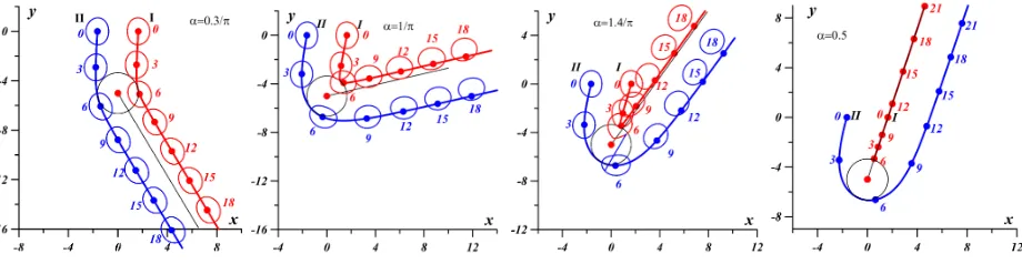
FIG. 2. (Color online) Scattering of a point-vortex pair impinging on a fixed point vortex. The ratio of the fixed vortex and pair circulationsαis shown in the frames. The fixed vortex is located atr0 = 5,θ0=−π/2. Pair’s vortices are initially located atx10=−x20= 1.65,y10=y20= 0 orr120 = 3.3, θ10= π₂ −0.319. The analogous finite size vortices have the same circulation ratio, the same initial positions and their areas equalπ. α= 0.3/π- small deflection as ∆ = 0_π.6(π−0.319)−π/2;α= 1/π - ∆ = 2_π(π−0.319)−π/2;α= 1.4/π - ∆ = 2_π.8(π−0.319)−π/2; complete reflection asα= 1/2 -∆ = (π−0.319)−π/2 =θ10. The black lines indicate scattering anglesθ1∞= 2α(π−0.319)−π/2. The black circle with radius 1.65 indicates the minimal permitted distance from the fixed vortex, the filled circles indicate the vortex positions at the given times.

To interpret these results, we write the value of 2αθ10 in the form

2α(π−∆θ0) = 2πn+ ∆. (15)

One can infer that one of pair’s vortices completesn−1/2 rotations around the fixed vortex, while the other one completesn+ 1/2 rotations. The scattering angle of the pair equals ∆. One can also obtain the minimal distance, which can possibly be attained between the moving vortices and the fixed vortex. This extremum of r1 can be found from eq. (11),

τm =

r2 120

2 cot (∆θ0), r1m =

r₁₂₀

2 . (16)

This means that the minimal distance from the fixed vortex to either of the moving ones is equal to half the initial distance between pair’s vortices.

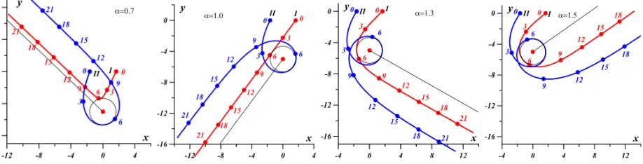
FIG. 3. (Color online) Same as in fig. 2 for different values ofα. α= 0.7 - small deflection after one half of a complete turn as ∆ = 1.4 (π−0.319)−π/2;α= 1 - one turn as ∆ = 2.0 (π−0.319)−π/2; α= 1.3 - small deflection after a complete turn as ∆ = 2.6 (π−0.319)−π/2;α = 1.5 - reflection after a complete turn as ∆ = 3.0 (π−0.319)−π/2 =θ10.

are performed using the contour dynamic techniques as in the work38_{. Detailed analysis of} the configuration using the finite-size vortex model is reported in the accompanying paper44_. The parameters used arer0 = 5, θ0 =−π/2,x10 =−x20 = 1.65, y10=y20 = 0 orr120 = 3.3,

θ10= π₂ −0.319, and the values of α are given in fig. 2.

Figure 2 shows a small deflection of the pair as it approaches the fixed vortex, followed by its reflection when α = 0.5. Figure 3 illustrates a similar deflection of the pair as it approaches the fixed vortex. In these cases, however, the pair is reflected after one half of a complete turn around the fixed vortex. The last panel of fig. 3 shows reflection after a complete turn. Figure 4 shows the reflection of the pair after two or three complete turns. The minimal distance between pair’s vortices and the fixed vortex is also indicated in the figures. It is worth mentioning that the scattering angle of the pair is independent of the initial distance separating its vortices.

The next section addresses the asymmetric case, i.e. when M ̸= 0. Now, the distance between pair’s vortices varies in time. The system therefore possesses no additional invariant.

IV. ASYMMETRIC CASE

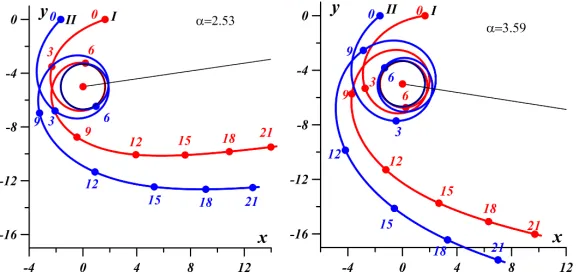
FIG. 4. (Color online) Same as in fig. 2 for relatively large values ofα. α= 2.53 near reflection after two complete turns as ∆ = 5.06 (π−0.319)−π/2; α = 3.59 near reflection after three complete turns as ∆ = 7.18 (π−0.319)−π/2.

periodically near the fixed vortex for an infinitely long time. This effect has an elegant application in physical oceanography. Indeed, the entrapping of coherent structures by a topographic feature is a common phenomenon in the ocean28,31,45–48_{. When this happens,} bounded motion of vortex structures may lead to effective passive scalar advection25,33,49.

We first analyze a necessary condition for the vortex pair to be entrapped near the fixed vortex. From eq. (4), it follows that pair’s vortices reach their extreme distances from the fixed vortex only when sin(θ1 − θ2) = 0, i.e. when both vortices are aligned along a straight line also passing through the fixed vortex. Without loss of generality, one can initially position pair’s vortices at the x-axis (see fig. 1). Furthermore, two configurations are possible: both vortices are initially aligned on one side of the fixed vortex (such that the distance between the vortices r12<max(r1, r2) ) or the fixed vortex lays between pair’s vortices (such that r12>max(r1, r2)). Hence,

r120 =r10+r20=re1+r

e

2, θ10−θ20=π,

r120 =|r10−r20|=|re1−r

e

2|, θ10−θ20 = 0.

(17)

Here, the superscript ’e’ denotes ’extreme value’. We choose the initial angles such that their difference,θ10−θ20, equals either zero orπand, consequently, there are extreme values

re

1, re2 of the radii for any initial value.

Substituting the extreme points r1 =r1e, r2 =re2 into eq. (6) results in

H2 =

H02

M =H2

±₌ (re1±re2) (re

1∓re2)

(

re

2

re

1

)2α

FIG. 5. (Color online) Extreme values ofH2 depending onρ1 – left panel; extreme values of −H2 depending on ρ2 – right panel. The curves corresponding to r12 = r1 ±r2 are indicated by the associated sign. α= 0.5.

the upper (lower) sign corresponds to θ1 −θ2 =π ( θ1−θ2 = 0,). This equation can be rewritten as follows

H2±= (1±ρe1)

(1∓ρe

1)

(ρe

1) 2α

, 0< ρ1 = r_r2₁ <1,

H2±= (ρe2±1) (ρe_2∓1)(ρ

e

2)

−2α

, 0< ρ2 = r_r1₂ <1,

(19)

where the superscript ’e’ again denotes ’extreme value’. Both cases are further addressed separately: r2 < r1 and r1 < r2. In the former case, one obtains

0< H2+=

(1 +ρe

1) (1−ρe

1)

(ρe₁)2α <∞, θ1−θ2 =π, 0< ρ1 <1;

0< H2−=

(1−ρe

1) (1 +ρe

1)

(ρe₁)2α <H¯2−, θ1−θ2 = 0, 0< ρ1 <1.

(20)

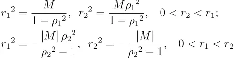
It is worth mentioning that the corresponding extrema of r1 and r2 denoted re1 and r2e respectively, are reached simultaneously at the extrema of the ratios ρ1andρ2. It is clearly seen from the general relations

r12 =

M

1−ρ12

, r22 =

M ρ12 1−ρ12

, 0< r2 < r1;

r12 =−

|M|ρ22

ρ22−1

, r22 =− |M| ρ22−1

, 0< r1 < r2.

One can easily calculate the second derivatives at the extreme points

¨

r1,2 = 1

r2 12re1,2

(

1±α

(

1

r −r

))

, cos (θ1−θ2) =±1, (r=r2eor r=−r

e

1).

Here, in the caseρ1,2 < ρ−1 =

(

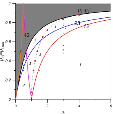
FIG. 6. Diagram of entrapment of the vortex pair. The grey area corresponds to entrapment, while the white area corresponds to unbounded motion to infinity.

value ofH2+ >0. The maxima of r1 and r2 are then attained when r12 =r1−r2 and exist only for a finite interval 0< H2− <H¯2−. If either of the ratios ρ1 or ρ2 tends to the value

ρ−₁, the maximal point transforms into an inflection point. The maximal value ¯H2− is

¯

H2−=

(

1−ρ−₁)

(

1 +ρ−₁)

(

ρ−₁)2α, ρ−₁ = −1 + √

1 + 4α2

2α . (21)

Figure 5 illustrates these dependencies. One can conclude that provided ρ1 not reaching its maximal value, the pair motion is unbounded. On the contrary, the pair can be entrapped in a bounded region for the parameters chosen under the line

H2(α) =

(

2α+ 1−√1 + 4α2)

(

2α−1 +√1 + 4α2)

(

−1 +√1 + 4α2 2α

)2α

(22)

in the plane (H2, α). The limiting curve of the bounded motion is shown in fig. 6. For the second case r1 < r2, we have

−∞< H2+ = (ρe

2+ 1) (ρe₂−1)(ρ

e

2)− 2α

<H¯2 +

, θ1−θ2 =π, 0< ρ2 =

r1

r2

<1;

−∞< H2− = (ρe

2−1) (ρe

2+ 1)

(ρe₂)−2α <0, θ1−θ2 = 0, 0< ρ2 =

r1

r2

<1.

(23)

Here, the minima of r1 and r2 are attained provided r12=r1−r2 and exist whenH2−<0. The maxima of r1 and r2 are then attained when r12=r1+r2 and exist only when −∞<

H2+<H¯2 +

. The maximal value ¯H2 + is ¯ H2 + = (

ρ+₂ + 1)

(

ρ+₂ −1)

(

ρ+₂)−2α, ρ+₂ =ρ−₁ = −1 + √

1 + 4α2

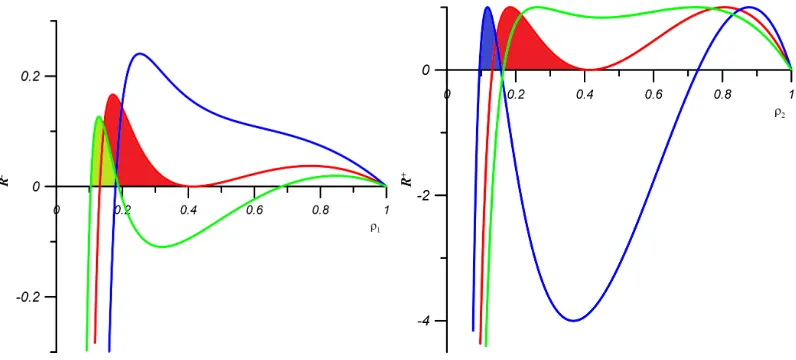
FIG. 7. (Color online) The radicand (26) depending on 0< r2

r1 <1 on the left panel and depending

on 0< r1

r2 <1 on the right one forα= 0.5. Regions of bounded motion are filled.

Figure 5 also illustrates these dependencies. Thus, provided ρ2 not reaching its maximal value, the motion of the pair is unbounded. This happens for the parameters chosen under the line

H2(α) =

(

−1 +√1 + 4α2_{+ 2α})

(

−1 +√1 + 4α2−_2α)

(

2α

−1 +√1 + 4α2

)2α

, (25)

in the plane (H2, α). The second limiting curve of unbounded motion is also shown in fig. 6.

Figure 7 illustrates the radicand from eq. (9) for values of H2 indicated in fig. 5 by horizontal lines. The radicand can be written in the form

R−= 1− 1 4

(

1

ρ1

+ρ1−

H02

M

(

1

ρ1 −

ρ1

)

(ρ1)−2α

)2

, 0< ρ1 <1,

R+= 1− 1 4

(

ρ2+ 1

ρ2 +H0

2

M (ρ2)

2α (

1

ρ2 −ρ2

))2

, 0< ρ2 <1,

(26)

Solutions of system (8) only exist provided ρ1 and ρ2 ensuring the positivity of the radicands. It is worth mentioning that if we exclude the symmetric case, the limits ρ1 → 1 and ρ2 → 1 are equivalent to the limits r1, r2 → ∞. Therefore one may infer from fig. 7 three regimes of motion for the pair. The motion is unbounded only for H2 > H¯2− and

ρ1 <1 or H2 <H¯2 +

and ρ2 <1.

Bounded motion of the pair happens given H2 < H¯2− and ρ1 < 1 or H2 > H¯2 +

and

radicands (26). The motion is again unbounded ifρ1 orρ2 are between the third zero of the radicands (26) and 1. The cases H2 = ¯H2− and ρ1 < 1 or H2 = ¯H2

+

and ρ2 < 1 separate the two types of motion. The critical points ρ−₁ or ρ+₂ are hyperbolic.

Before considering the trajectories permitted for the pair, we examine the frequencies of the bounded motion. System (4) has two intrinsic periods. The first one is the period of rotation of pair’s vortices about the fixed vortex. To estimate this period, we rewrite eq. (4) as

˙

θ1 =− 1

M

1−ρ1cos (θ1−θ2)

r2 12/M

+ α

M

(

1−ρ12

)

, θ˙2 = 1

M

ρ1−cos (θ1−θ2)

ρ1r212/M

+ α

M

1−ρ12

ρ12 ;

˙

θ1 =− 1

M

ρ2−cos (θ1 −θ2)

ρ2r122 /M

+ α

M

ρ22−1

ρ22

, θ˙2 = 1

M

1−ρ2cos (θ1−θ2)

r2 12/M

+ α

M

(

ρ22−1

)

.

(27) One can calculate the angular velocities when the vortices attain the extreme points. We start with the case r2 < r1. Given the initial values of r1, r2 such that ρ1+ < ρ1 min < ρ1 =

ρ1 max < ρ1−, the angular velocities of the vortices at the maximal positions are

˙

θ1 = [α(1−ρ1 max)−1]

(1 +ρ1 max)

M ,

˙

θ2 =

[

α(1−ρ1 max) ρ1 max

−1

]

(1 +ρ1 max)

M ρ1 max

.

(28)

The angular velocities at the maxima ofr1, r2 vanish when the parameterαand initial ratio

ρ1 max comply with

α= 1

1−ρ1 max

(or ρ1 max =

α−1

α ) (29)

for the first vortex, and with

α= ρ1 max 1−ρ1 max

(or ρ1 max =

α

1 +α) (30)

for the second one. It follows that the angular velocities at the maxima of r1, r2 change signs when one chooses parametersα, ρ1 max below or above the curves from eqs. (29), (30), shown in fig. 8.

The minimum of ρ1 lead correspondingly to

˙

θ1 = [α(1 +ρ1 min)−1]

(1−ρ1 min)

M ,

˙

θ2 =

[

α(1 +ρ1 min) ρ1 min

+ 1

]

(1−ρ1 min)

M ρ1 min

.

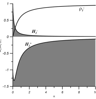
FIG. 8. (Color online) Permitted motion regimes of pair’s vortices for various values of the pa-rameterα and initial ratio ρ(1,2) max. The pair moves in a bounded area for the parameters taken below the bold black line. The first vortex has a positive angular velocity at the maximal position for the parameters taken below the red (marked as 12) line (29) and, conversely, a negative angu-lar velocity for the parameters taken above the line. At the minimum, this vortex has a positive angular velocity to the right of the magenta (marked as 42) line (32) and, conversely, a negative angular velocity - to the left. The second vortex has a positive angular velocity at the maximum for the parameters taken below the blue (marked as 23) line (30) and, conversely, a negative angular velocity - above it. At the minimum, this vortex has always a positive angular velocity because the demarcating line (33) lays beyond this area. The orange (marked asI) line corresponds to the eq. (35). The dashed line depicts the cases when the first vortex’s averaged angular velocity equals zero <θ˙1 >T= 0 (hereT is the period of pair’s oscillations). The isolated dots correspond to the

vortex trajectories shown further forr2< r1 – red dots and forr1 < r2 – blue dots.

It is worth noticing that ρ1 min is uniquely defined byρ1 max. The same is valid for ρ2 min and ρ2 max. This comes from analyzing fig. 5. The angular velocities at the minima ofr1, r2 vanish when the parameter α and initial ratio ρ1 max satisfy

α= 1

1 +ρ1 min

(or ρ1 min= 1−α

α ) (32)

for the first vortex, and

α =− ρ1 min 1 +ρ1 min

(or ρ1 min=−

α

for the second one. The curve (33) is beyond the physical domain, so the second vortex’s angular velocity does not change the sign at the minimum. The angular velocity of the first vortex changes its sign at the minima of r1, r2 when one takes the parameters α, ρ1 max bellow or above the curves from eq. (32), shown in fig. 8.

Furthermore, five possible qualitative types of the pair trajectories ensue depending on the parameter α and the initial value of the ratio ρ1 max < ρ1−.

1. Both vortices move counter-clockwise (both angular velocities are positive) at the maximal and at the minimal positions (see fig. 9).

2. The angular velocity of the first vortex at the maximal position is negative, while at the minimum position it is positive. The angular velocity of the second vortex is positive at the maximum and minimum positions (see fig. 11).

3. The angular velocity of both vortices are negative at the maximal positions, and, oppositely, positive at the minimal positions (see fig. 12).

4. The angular velocity of the first vortex is negative, while the angular velocity of the second vortex is positive for all time. See fig. 10.

5. The angular velocity of the first vortex is negative for all time, while the angular velocity of the second vortex is negative at the maximal position and positive at the minimal position (see fig. 13).

We next explore the case r1 < r2. Given the maximal value of ρ2− < ρ2 min < ρ2 =

ρ2 max < ρ2+, one obtains

˙

θ1 =

(

αρ2 max+ 1 ρ2 max

−1

)

1−ρ2 max |M|ρ2 max

,

˙

θ2 = (α(ρ2 max+ 1) + 1)

1−ρ2 max |M| .

(34)

These relations suggest that the angular velocity of the first vortex at the maximum changes its sign when one takes the parameters α, ρ2 max above or bellow the line

α= ρ2 max

ρ2 max+ 1

. (35)

angular velocity of the second vortex also never changes its sign at the maximum. The curve (35) is shown in fig. 8.

For the minimal values of ρ2, one obtains

˙

θ1 = 1 |M|

(

1 +α1−ρ2 min ρ2 min

)

ρ2 min+ 1

ρ2 min

,

˙

θ2 = 1

|M|(1 +α(1−ρ2 min)) (ρ2 min+ 1).

(36)

The angular velocity of both vortices never changes its sign at the minimal position. Thus, only one possible type of the vortex trajectories occurs. The vortices rotate counter-clockwise for all time, with slightly changing their angular velocities. It is worth noticing that the rotational periods of the vortices, 2π/⟨θ1⟩,2π/⟨θ2⟩, are inherently of the same time-scale. Indeed, one can recast them in the form,

⟨θ1⟩=⟨θ2⟩+ 2πn, (37)

where n depends on the type of the trajectories shown in fig. 8, and < . > stands for the averaging over one period of the first vortex rotation about the fixed vortex.

Furthermore, the system possesses a second time-scale, that is a time period during which r1, r2 pass between their extreme positions. This second time scale can be found by averaging the angular velocity from eq. (8). Provided ρ1 max ≪ 1 or ρ2 max ≪ 1, one can estimate these frequencies

˙

θ1−θ˙2 ˙

θ1

∼ − α

α−1

(

1

ρ1 max

)2

,

˙

θ1−θ˙2 ˙

θ2

∼ −1, 0< r2 ≪r1;

˙

θ1−θ˙2 ˙

θ1

∼1,

˙

θ1−θ˙2 ˙

θ2

∼ α

α+ 1

(

1

ρ2 max

)2

, 0< r1 ≪r2.

(38)

The next step is to analyze the angular velocities given the ratio ρ1 or ρ2 being close to the separatrix values ρ1− or ρ2+. By linearizing eq. (8) near these points and assuming (ρ1 =ρ1−+ρ,θ1−θ2 =θ) or (ρ2 =ρ2++ρ,θ1−θ2 =π+θ), withρandθ being infinitesimal, one obtains the system

˙

ρ= _M1 (1 +ρ1−) 2

θ,

˙

θ= (1−ρ1

2₎

M ρ1−2 (2αρ1

−_{+ 1)ρ,} 0< r2 < r1;

d dtρ=

1

M(1−ρ2

+₎2_θ, ˙

θ= (1−ρ2

+2₎

M ρ2+2 (2αρ2

+_{+ 1)ρ,} 0< r1 < r2.

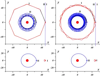
FIG. 9. (Color online) Vortex trajectories of the first vortex (red) and second vortex (dark blue) for the bounded motion case corresponding to regime 1 in fig. 8; and the first vortex (magenta) and second vortex (blue) for the unbounded motion case associated with the same value of H2 as is in the bounded case. α = 3, r10 = 50.0, θ10 = θ20 = 0. Top row: (left) – r_r20₁₀ = 0.5045 (⟨θ˙_⟨1−_˙θ˙2⟩

θ1⟩ = 8); (right) –

r20

r10 = 0.52, (7<

⟨_θ˙_1−θ˙₂⟩

⟨_θ˙₁⟩ <8 ). Bottom row: same as in the top row, except in a coordinate system rotating with the angular velocity

⟨

˙ θ1−θ˙2

⟩

. The black segments of the trajectories show the first period ofr1, r2.

The relations imply that the points (ρ1−,0) and (ρ2+, π) are hyperbolic. Therefore, the frequency

⟨

˙

θ1−θ˙2

⟩

is zero at this phase trajectory. Nevertheless, the average rotation

frequency of either vortex,

⟨

˙

θ1

⟩

and

⟨

˙

θ2

⟩

, near these hyperbolic points remains finite.

A. Numerical results

The purpose of this section is to illustrate vortex trajectories for different values of the angular velocity. We start with the case 0< ρ1 <1.

(in terms of angular velocity). In case 1, both vortices move counter-clockwise for all time. In case 4, the first vortex moves clockwise, and the second vortex moves counter-clockwise for all time. Probing the ratio of the inherent time-scales, it follows from the estimates eq. (38) that given ρ1 max<< 1, the first vortex moves significantly slower than the second one and even in comparison with the pair rotation period 2π/

⟨

˙

θ1−θ˙2

⟩

. One can conclude that there are many maxima and minima of r1, r2 while the first vortex completes one turn around the fixed vortex. However, both vortices reach their extreme positions concurrently. The estimates eq. (38) ensure that the second vortex turns with the first one on the same angle and completes another turn around the fixed vortex during one oscillation period of the pair.

This situation is illustrated in fig. 9 and 10. The first period of pair rotation, 2π/

⟨

˙

θ1−θ˙2

⟩

, is indicated by a bold black line to show the direction of the vortex rotation. Another feature is that the vortex trajectories are always periodic in the reference frame rotating with the angular velocity

⟨

˙

θ1−θ˙2

⟩

. This property is also shown in the figures. The next feature worth noticing is the decrease of the angular velocity of the first vortex when α ∼1. This comes from the estimate (38). Although the estimate is not strictly valid for this value ofα, it provides a qualitative tendency. The same conclusion can be inferred from eq. (28),(31) or (27). This fact further transpires when considering motion of type 2 shown in fig. 8.

When the parameters correspond to the second and third motion types, the angular velocity of the first vortex changes its sign when the pair passes between its extreme positions. This means that the averaged angular velocity of the first vortex,

⟨

˙

θ1

⟩

, can be zero. The

line in the diagram of fig. 8 corresponding to the

⟨

˙

θ1

⟩

(α, ρ1 max) = 0 now starts at the point

α= 1, ρ1 max= 0 and remains in regions 2 and 3. Numerically calculated, this dashed line is plotted in fig. 8. The line has no stagnation points because

⟨

˙

θ2

⟩

(α, ρ1 max) = 2π, provided

⟨

˙

θ1

⟩

(α, ρ1 max) = 0.

We next consider permitted values of the ratio ⟨θ˙_⟨1−_˙θ˙2⟩

θ1⟩ as the parameters vary. The ratio

tends to infinity when ρ1 max → 0. This case is illustrated in fig. 9 and fig. 10. There is a minimum between the region for smallρ1 and the line

⟨

˙

θ1

⟩

(α, ρ1) = 0. Specifically, whenα

is sufficiently large, the curve

⟨

˙

θ1

⟩

(α, ρ1) = 0 lays in region 3 shown in fig. 8; moreover, the

minimum of the ratio ⟨θ˙_⟨1−_˙θ˙2⟩

θ1⟩ coincides with the one attained in region 2. Here only a small

range where ratio ⟨θ˙_⟨1−_˙θ˙2⟩

θ1⟩ changes. For example, forα = 3 we have 5<

⟨_θ˙_1−θ˙₂⟩

FIG. 10. (Color online) Same as in fig. 9 corresponding to region 4 from fig. 8. α= 0.5,r10= 50.0, θ10 = θ20 = 0. Left – r_r20₁₀ = 0.3185 (⟨

˙

θ1−θ˙2⟩

⟨_θ˙₁⟩ = 11); right – same as to the left, but plotted in a rotating reference frame of the angular velocity

⟨

˙ θ1−θ˙2

⟩

. The black segments of the trajectories indicate the first oscillation period of r1, r2.

shown in fig. 8. Thus, periodic trajectories exist only for specific values ofα, provided that it is sufficiently large. Figure 11 depicts this case.

The final feature to notice concerns the ratio of the angular velocities near the separatrix as ρ1 max → ρ1−. The pair rotation period tends to infinity when ρ1 max → ρ1−. Thus, the ratio ⟨θ˙_⟨1−_˙θ˙2⟩

θ1⟩ tends to infinity given ρ1 max →0 and near the curve ⟨

˙

θ1

⟩

(α, ρ1 max) = 0, and, inversely, tends to zero as ρ1 max →ρ1−.

Furthermore, the ratio ⟨θ˙_⟨1−_˙θ˙2⟩

θ1⟩ can in particular be rational or natural. Both cases ensure

that the vortex trajectories are periodic in the original non-rotating reference frame. This is also shown in fig. 9 – 13. The case when

⟨

˙

θ1

⟩

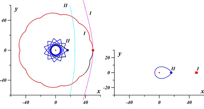
(α, ρ1 max) = 0 belonging to region 2 is also illustrated in fig. 11. The right bottom panel shows the case when the counter-clockwise and clockwise rotation exactly compensate each other. This case is of particular interest because the first vortex never rotates about the fixed vortex and only oscillates in a small bounded region.

We next describe the types of motion close to the separatrix, i.e. types 3 and 5 shown in fig. 8. An example of vortex trajectories characterized by the type 3 motion is illustrated in fig. 12. The top left panel depicts an increase of the ratio ⟨θ˙_⟨1−_˙θ˙2⟩

θ1⟩ compared to the top

left panel in fig. 11. The top right panel corresponds to the case

⟨

˙

θ1

⟩

FIG. 11. (Color online) Same as in fig. 9 for region 2 shown in fig. 8. r10= 50.0, θ10=θ20 = 0. Top: (left) – α= 3.1325, r20

r10 = 0.74 (

⟨_θ˙_1−θ˙₂⟩

⟨_θ˙₁⟩ = 5), (right) -α = 0.9, rr2010 = 0.4175 (

⟨_θ˙_1−θ˙₂⟩

⟨_θ˙₁⟩ = 21); bottom: (left) – same as in the top (left) panel but plotted in a rotating reference frame of the angular velocity

⟨

˙ θ1−θ˙2

⟩

, (right) - α = 1.2268, r20

r10 = 0.4 (

⟨_θ˙₁⟩

⟨_θ˙_1−θ˙₂⟩ = 0). The black trajectory segments indicate the first oscillation period ofr1, r2.

first vortex is not rotating about the fixed vortex. The bottom panels show a decrease of the ratio ⟨θ˙_⟨1−_˙θ˙2⟩

θ1⟩ asρ1 max tends toρ1 −_.

The motion type corresponding to region 5 differs from the one associated with region 3 as is exemplified by fig. 13. This region corresponds to the first vortex always moving clockwise. As the ratio ⟨θ˙1−θ˙2⟩

⟨_θ˙₁⟩ approaches the separatrix, it decreases leading to the appearance of special trajectories of the second vortex. Indeed, as has been shown above,θ2(T = _⟨θ˙₁₋2π_θ˙₂⟩) =

θ1(T) + 2π, however, given the parameters ρ1 max = 0.41421,α = 0.5, one arrives atθ1(T) = −2π and

⟨

˙

θ2

⟩

= 0. This implies that the second vortex may not necessarily complete a full rotation about the fixed vortex.

The next case to consider corresponds to 0 < r1

r2 <1. The vortices always rotate

counter-clockwise. Therefore, no solutions are permitted given

⟨

˙

θ1

⟩

= 0 or

⟨

˙

θ2

⟩

FIG. 12. (Color online) Same as in fig. 9 corresponding to region 3 shown in fig. 8. α = 3.0, r10 = 50.0, θ10 = θ20 = 0. Top: (left) – r_r20₁₀ = 0.7714 (⟨

˙

θ1−θ˙2⟩

⟨_θ˙₁⟩ = 6), (right) –

r20

r10 = 0.83505

(_⟨˙⟨θ˙1⟩

θ1−θ˙2⟩ = 0); bottom: (left) –

r20

r10 = 0.8465 (

⟨_θ˙_1−θ˙₂⟩

⟨_θ˙₁⟩ = 3), (right) –

r20

r10 = 0.8471 (

⟨_θ˙_1−θ˙₂⟩ ⟨_θ˙₁⟩ = 1). The black trajectory segments mark the first oscillation period of r1, r2 in the left top panel and half of a period for the remaining panels.

the ratio ⟨θ˙_⟨1−_˙θ˙2⟩

θ1⟩ decreases at a much faster rate as the parameters approach the separatrix

curve ρ2+(α). Exemplary trajectories are shown in fig. 14,15. The ratio ⟨ ˙

θ1−θ˙2⟩

⟨_θ˙₁⟩ < 1 is shown in fig. 15. The right panel of fig. 15 illustrates an example of motion occurring near the separatrix over a long time. When the ratio ⟨θ˙_⟨1−_˙θ˙2⟩

θ1⟩ < 1, the vortices move from

FIG. 13. (Color online) Same as in fig. 9 corresponding to region 5 shown in fig. 8. α = 0.5, r10= 50.0,θ10=θ20= 0. Left – r_r20₁₀ = 0.3508 (⟨

˙

θ1−θ˙2⟩

⟨_θ˙₁⟩ = 8), (right) – rr2010 = 0.41421 (

⟨_θ˙_1−θ˙₂⟩ ⟨_θ˙₁⟩ = 1). The trajectory black segments mark the first period of r1, r2 in the left panel and half a period in the right one.

V. CONCLUSIONS

The dynamics of a vortex pair consisting of two equal counter-rotating point vortices that impinges on a fixed point vortex in a homogeneous barotropic fluid has been analyzed in detail. A paper upon which the present study has been based24 _{categorizes the possible} motion into two types: (i) symmetric case: pair’s vortices are located at the same (variable) distance from the fixed vortex, which makes the pair always scatter and move unbound-edly when approaching the fixed vortex; (ii) asymmetric case: the distances between pair’s vortices and the fixed vortex are not equal, and the motion of pair’s vortices can be bounded. Results for the symmetric case have been refined and preliminary calculations for an analogous finite area vortex model have been illustrated. These calculations have been carried out by the method of contour dynamics38 _{and agree well with the dynamics of the} point-vortex model.

FIG. 14. (Color online) Trajectories of the first (red) and second (dark blue) vortices for bounded motion, and of the first (magenta) and second (blue) vortices for unbounded motion given the same values of H2: θ10 =π, θ20 = 0, r20 = 50.0. Top row: (left) – α = 0.5, r_r10₂₀ = 0.297 ( ⟨

˙

θ1−θ˙2⟩

⟨_θ˙₂⟩ = 5, ⟨_θ˙₂⟩

⟨_θ˙₁⟩ = 1

5+1); (right) –α = 1.5,

r10

r20 = 0.296 (

⟨_θ˙_1−θ˙₂⟩ ⟨_θ˙₂⟩ = 8 ,

⟨_θ˙₂⟩ ⟨_θ˙₁⟩ =

1

8+1 ). Bottom row α= 3.0: (left) – r20

r10 = 0.482, (

⟨_θ˙_1−θ˙₂⟩ ⟨_θ˙₂⟩ = 3,

⟨_θ˙₂⟩ ⟨_θ˙₁⟩ =

3

3+1), (right) –

r10

r20 = 0.561 (

⟨_θ˙_1−θ˙₂⟩

⟨_θ˙₂⟩ = 2 ). The trajectory black segments denominate the first oscillation period of r1, r2.

bounded and unbounded motion regimes has been derived.

FIG. 15. (Color online) Same as in fig. 14. α= 3.0,r20= 50.0,θ10=π, θ20= 0. Left – r_r10₂₀ = 0.69 (⟨θ˙_⟨1−_˙θ˙2⟩

θ2⟩ = 1,

⟨_θ˙₂⟩

⟨_θ˙₁⟩ = 1+11 ), right

-r20

r10 = 0.82 (

⟨_θ˙_1−θ˙₂⟩ ⟨_θ˙₂⟩ = 13,

⟨_θ˙₂⟩

⟨_θ˙₁⟩ = 3+13 ). The trajectory black segments mark the first half of the period of r1, r2.

vortex trajectories. An important feature is that there is a separatrix delineating bounded and unbounded motion regimes. The availability of a hyperbolic point and the separatrix makes it promising to perturb the regular steady–state to look into nascent chaotic dynamics. Another interesting feature of the pair bounded motion is that the system possesses two proper frequencies. The first one is the pair oscillation frequency and the second one is the frequency of the pair rotation around the fixed vortex. The permitted frequencies range from 0 to infinity, which may be facilitating in order to obtain an abundance of chaotic dynamics regimes50–53.

Making use of the intrinsic frequencies, one can pass over to a rotating reference frame in which one of the vortices will not rotate about the fixed vortex. If the parameters and initial vortex positions result in the fact that the ratio of the frequencies is a rational or natural number, the vortex trajectories are periodic in the original reference frame. A number of configurations that feature one vortex not rotating about the fixed vortex has been found.

model that accounts for the fact that the vortices may significantly alter their shape when interacting with each other. Therefore, the second part of the study is intended to demon-strate complicated vortex dynamics found in the finite area vortex model that is similar to the one permitted by the analogous point-vortex model and reported here.

As a final remark, we would like to mention that the model in question might be of use not only for hydrodynamic applications but also in physics of superfluids. For instance, configurations of similar coherent structures have been extensively analyzed in context of Bose-Einstein condensates54–56_.

ACKNOWLEDGMENTS

The reported study was partially supported the POI FEB RAS Program ”Mathematical simulation and analysis of dynamical processes in the ocean” (117030110034−7) and by the Russian Foundation for Basic Research, project no. 17−05−00035. EAR was partially sup-ported by the NERC grant N E/R011567/1. The work of KVK in obtaining the analytical estimates was supported by the Russian Scientific Foundation, project no. 16−17−10025.

VI. APPENDIX. ANOTHER REPRESENTATION OF THE SYMMETRIC

CASE SOLUTION

Let us derive the equation for r1 from (4) for the symmetric case, i.e. r12is constant and

r1 =r2. Hence

¨

r1 = 1

r₁₂2

(

˙

r1sin (θ1−θ2) +r1cos (θ1−θ2)

(

˙

θ1−θ˙2

))

.

This equation can be rewritten in the form

˙

r1¨r1 = 1 2

d dτr˙

2 1 =

˙

r1 4r3

1

=− d

dτ

1 8r2

1

.

Integrating this equation results in

r1 =

r12 2

(

1 + 4

r4 12

(τ −τm)2 )1/2

; τm =−r˙10r10r122 =−r102sin (θ10−θ20),

where we use the equality 1 + 4 ˙r2

10r210 = (2r10/r12)2. From this it follows that r1 has a minimum at r12

By inserting the solutionr1 inside the evolution equation for

(

˙

θ1−θ˙2

)

(12) and integrat-ing, one arrives at

θ1(t)−θ2(t)

2 =

θ10−θ20

2 −arctan

(

2

r2 12

(τ −τm) )

+ (2α−1) arctan

(

2

r2 12

τm )

,

θi(t) =θi0+ (2α∓1)

(

arctan

(

2

r2 12

(τ−τm) )

+ arctan

(

2

r2 12

τm ))

, (i= 1,2).

In certain cases, this form of the solutions is more convenient than the one presented in the paper’s main body.

REFERENCES

1_{H. Aref, N. Rott, and H. Thomann, “Gr¨obli’s solution of the three-vortex problem,” Annu.}

Rev. Fluid Mech. 24, 1–20 (1992).

2_{P. G. Saffman, Vortex dynamics (Cambridge University Press, Cambridge, 1992).}

3_{B. A. Klinger, “Baroclinic eddy generation at a sharp corner in a rotating system,” J.}

Geophys. Res. 99, 12515–12531 (1994).

4_{A. Borisov and I. Mamaev, Mathematical methods in the dynamics of vortex structures}

(Institute of Computer Science, MoscowIzhevsk, 2005).

5_{V. Meleshko and H. Aref, “A bibliography of vortex dynamics 1858–1956,” Adv. Appl.}

Mech. 41, 197–292 (2007).

6_{M. A. Sokolovskiy and J. Verron, Dynamics of vortex structures in a stratified rotating}

fluid (Springer, Switzerland, 2014).

7_{O. R. Southwick, E. R. Johnson, and N. R. McDonald, “A simple model for sheddies:}

Ocean eddies formed from shed vorticity,” J. Phys. Oceanogr. 46, 2961–2979 (2016). 8_{M. Sokolovskiy, K. Koshel, and J. Verron, “Three-vortex quasi-geostrophic dynamics in}

a two-layer fluid. Part 1. Analysis of relative and absolute motions,” J. Fluid Mech. 717, 232–254 (2013).

9_{K. V. Koshel, M. A. Sokolovskiy, and J. Verron, “Three-vortex quasi-geostrophic dynamics}

in a two-layer fluid. Part 2. Regular and chaotic advection around the perturbed steady states,” J. Fluid Mech. 717, 255–280 (2013).

10_{B. Shteinbuch-Fridman, V. Makarov, X. Carton, and Z. Kizner, “Two-layer geostrophic}

11_{B. Shteinbuch-Fridman, V. Makarov, and Z. Kizner, “Transitions and oscillatory regimes}

in two-layer geostrophic hetons and tripoles,” J. Fluid Mech. 810, 535–553 (2017). 12_{J. Synge, “On the motion of three vortices,” Can. J. Math 1, 257–270 (1949).} 13_{H. Aref, “Motion of three vortices,” Phys. Fluids 22, 393–400 (1979).}

14_{H. Aref, “Integrable, chaotic, and turbulent vortex motion in two-dimensional flows,”}

Annu. Rev. Fluid Mech. 15, 345–389 (1983).

15_{H. Aref, “Three-vortex motion with zero total circulation: Addendum.” J. Appl. Math.}

Phys. (ZAMP) 40, 495–500 (1989).

16_{X. Leoncini, L. Kuznetsov, and G. Zaslavsky, “Motion of three vortices near collapse,”}

Phys. Fluids 12, 1911–1927 (2000).

17_{C. K. Taylor and S. G. Llewellyn Smith, “Dynamics and transport properties of three}

surface quasigeostrophic point vortices,” Chaos 26, 113117 (2016).

18_{V. M. Gryanik and M. V. Tevs, “Dynamics of singular geostrophical vortices in a n-level}

model of the atmosphere (ocean),” Izv. Atmos. Ocean. Phys. 25, 179–188 (1989). 19_{P. K. Newton, The N-vortex problem: analytical techniques (Springer, 2001).}

20_{V. M. Gryanik, M. A. Sokolovskiy, and J. Verron, “Dynamics of heton-like vortices,”}

Regul. Chaotic Dyn. 11, 383–434 (2006).

21_{X. Perrot and X. Carton, “Point-vortex interaction in an oscillatory deformation field:}

Hamiltonian dynamics, harmonic resonance and transition to chaos,” Discrete Cont. Dyn.-B 11, 971–995 (2009).

22_{O. R. Southwick, E. R. Johnson, and N. R. McDonald, “A point vortex model for the}

formation of ocean eddies by flow separation,” Phys. Fluids 27, 016604 (2015).

23_{G. G. Sutyrin, X. Perrot, and X. Carton, “Integrable motion of a vortex dipole in an}

axisymmetric flow,” Phys. Lett. A 372, 5452–5457 (2008).

24_{E. A. Ryzhov and K. V. Koshel, “Dynamics of a vortex pair interacting with a fixed point}

vortex,” EPL 102, 44004 (2013).

25_{E. A. Ryzhov, “Irregular mixing due to a vortex pair interacting with a fixed vortex,”}

Phys. Lett. A 378, 3301–3307 (2014).

26_{J. Verron, “Topographic eddies in temporally varying oceanic flows,” Geophys. Astrophys.}

Fluid Dyn. 35, 257–276 (1986).

27_{M. E. Stern, “Scattering of an eddy advected by a current towards a topographic obstacle,”}

28_{W. K. Dewar, “Baroclinic eddy interaction with isolated topography,” J. Phys. Oceanogr.}

32, 2789–2805 (2002).

29_{M. Budyansky, M. Uleysky, and S. Prants, “Hamiltonian fractals and chaotic scattering}

of passive particles by a topographical vortex and an alternating current,” Physica D195, 369–378 (2004).

30_{V. N. Zyryanov, “Topographic eddies in a stratified ocean,” Regul. Chaotic Dyn. 11,}

491–521 (2006).

31_{R. Iacono, “Stable shallow water vortices over localized topography,” J. Phys. Oceanogr.}

40, 1143–1150 (2010).

32_{E. A. Ryzhov and K. V. Koshel, “Estimating the size of the regular region of a}

topograph-ically trapped vortex,” Geophys. Astrophys. Fluid Dyn. 105, 536–551 (2011).

33_{E. A. Ryzhov and K. V. Koshel, “Interaction of a monopole vortex with an isolated}

topo-graphic feature in a three-layer geophysical flow,” Nonlin. Processes Geophys. 20, 107–119 (2013).

34_{I. Bashmachnikov, C. M. Loureiro, and A. Martins, “Topographically induced circulation}

patterns and mixing over Condor seamount,” Deep Sea Res. 98, 38–51 (2013).

35_{G. S. Deem and N. J. Zabusky, “Vortex waves–stationary V–states, interactions,}

recur-rence, and breaking,” Phys. Rev. Lett. 40, 859–862 (1978).

36_{P. Luzzatto-Fegiz and C. H. K. Williamson, “An efficient and general numerical method}

to compute steady uniform vortices,” J. Comput. Phys. 230, 6495–6511 (2011).

37_{V. G. Makarov, M. A. Sokolovskiy, and Z. Kizner, “Doubly symmetric finite-core heton}

equilibria,” J. Fluid Mech. 708, 397–417 (2012).

38_{J. N. Reinaud, M. A. Sokolovskiy, and X. Carton, “Geostrophic tripolar vortices in a}

two-layer fluid: Linear stability and nonlinear evolution of equilibria,” Phys. Fluids 29, 036601 (2017).

39_{J. N. Reinaud, M. A. Sokolovkiy, and X. Carton, “Hetonic quartets in a two-layer}

quasi-geostrophic flow: V–states and stability,” Physics of Fluids 30, 056602 (2018).

40_{G. Riccardi, “A complex analysis approach to the motion of uniform vortices,” Ocean}

Dynamics 68, 273293 (2018).

41_{E. A. Ryzhov and M. A. Sokolovskiy, “Interaction of a two-layer vortex pair with a}

1868–1882 (1975).

43_{G. M. Zaslavsky, The Physics of Chaos in Hamiltonian Systems (Imperial College Press,}

London, 2007).

44_{J. N. Reinaud, K. V. Koshel, and E. A. Ryzhov, “Dynamics of a vortex pair interacting}

with a fixed point vortex revisited. Part II: Finite size vortices,” Phys. Fluids submitted

(2018).

45_{J. Allen, R. M. Samelson, and P. Newberger, “Chaos in a model of forced quasi-geostrophic}

flow over topography : an application of melnikov’s method,” J. Fluid Mech.226, 511–547 (1991).

46_{P. G. Baines, Topographic effects in stratified flows (Cambridge University Press, 1993).} 47_{E. Kunze and J. M. Toole, “Tidally driven vorticity, diurnal shear, and turbulence atop}

fieberling seamount,” J. Phys. Oceanogr. 27, 2663–2693 (1997).

48_{J. Ledwell, E. Montgomery, K. Polzin, L. St Laurent, R. Schmitt, and J. Toole, “Evidence}

for enhanced mixing over rough topography in the abyssal ocean,” Nature 403, 179–182 (2000).

49_{E. A. Ryzhov and K. V. Koshel, “Ventilation of a trapped topographic eddy by a captured}

free eddy,” Izv. Atmos. Ocean. Phys. 47, 780–791 (2011).

50_{K. V. Koshel, M. A. Sokolovskiy, and P. A. Davies, “Chaotic advection and nonlinear}

resonances in an oceanic flow above submerged obstacle,” Fluid Dyn. Res. 40, 695–736 (2008).

51_{E. Ryzhov, K. Koshel, and D. Stepanov, “Background current concept and chaotic}

ad-vection in an oceanic vortex flow,” Theor. Comput. Fluid Dyn. 24, 59–64 (2010).

52_{E. A. Ryzhov and K. V. Koshel, “Global chaotization of fluid particle trajectories in a}

sheared two-layer two-vortex flow,” Chaos 25, 103108 (2015).

53_{E. A. Ryzhov and K. V. Koshel, “Resonance phenomena in a two-layer two-vortex shear}

flow,” Chaos 26, 113116 (2016).

54_{L. A. Smirnov and A. I. Smirnov, “Scattering of two-dimensional dark solitons by a single}

quantum vortex in a Bose–Einstein condensate,” Phys. Rev. A 92, 013636 (2015).

55_{L. A. Smirnov, A. I. Smirnov, and V. A. Mironov, “Scattering of a vortex pair by a single}

quantum vortex in a Bose–Einstein condensate,” JETP 149, 23–40 (2016).

56_{A. Griffin, G. W. Stagg, N. P. Proukakis, and C. F. Barenghi, “Vortex scattering by}