ISSN Print: 2161-718X
DOI: 10.4236/ojs.2019.96040 Nov. 26, 2019 623 Open Journal of Statistics
Likelihood Methods for Basic Stratified
Sampling, with Application to Von Bertalanffy
Growth Model Estimation
Nan Zheng, Noel Cadigan
Centre for Fisheries Ecosystems Research, Fisheries and Marine Institute of Memorial University of Newfoundland, St. John’s, NL, Canada
Abstract
This paper mainly addresses maximum likelihood estimation for a re-sponse-selective stratified sampling scheme, the basic stratified sampling (BSS), in which the maximum subsample size in each stratum is fixed. We derived the complete-data likelihood for BSS, and extended it as a full-data likelihood by incorporating incomplete data. We also similarly extended the empirical proportion likelihood approach for consistent and efficient estima-tion. We conducted a simulation study to compare these two new approaches with the existing estimation methods in BSS. Our result indicates that they perform as well as the standard full information likelihood approach. Me-thods were illustrated using a growth model for fish size at age, including between-individual variability. One of our major conclusions is that the fully observed BSS data, the partially observed data used for stratification, and the sampling strategy are all important in constructing a consistent and efficient estimator.
Keywords
Length-Stratified Age Sampling, Response-Selective Sampling, Basic Stratified Sampling, Complete-Data Likelihood, Empirical Proportion Likelihood
1. Introduction
In stratified random sampling (SRS), the population or a random sample of the population is partitioned into relatively homogeneous subgroups, or strata, and then random samples are taken independently in each stratum for full observa-tion. Such sampling design may also be regarded as a kind of two-phase sam-How to cite this paper: Zheng, N. and
Cadigan, N. (2019) Likelihood Methods for Basic Stratified Sampling, with Application to Von Bertalanffy Growth Model Estima-tion. Open Journal of Statistics, 9, 623-642.
https://doi.org/10.4236/ojs.2019.96040 Received: October 31, 2019
Accepted: November 23, 2019 Published: November 26, 2019
Copyright © 2019 by author(s) and Scientific Research Publishing Inc. This work is licensed under the Creative Commons Attribution International License (CC BY 4.0).
DOI: 10.4236/ojs.2019.96040 624 Open Journal of Statistics
pling, with the population or the large sample before partitioning being the first phase sample, and the smaller and more extensive subsamples after partitioning being the second phase samples.
Practical implementations of SRS frequently fall into two categories as classi-fied by [1]: 1) basic stratified sampling (BSS) where the maximum second phase subsample size (BSS1) or subsampling fraction (BSS2) in each stratum is pre-fixed, and 2) variable probability sampling (VPS) in which sequential units are independently generated from a model and then classified into strata where they are selected for full observation with pre-specified probabilities. [2] classified BSS2 as VPS, and hence all the inference methods for VPS are also suitable for BSS2.
Assume that there are a total of N sampling units on which the stratified sam-pling is conducted. Let yi and xi, i=1, , N, denote respectively the vectors
of responses and covariates of the ith individual generated from the joint distri-bution f
(
y x, |θ)
=g(
y x| ;θ) ( )
h x , withθ
being a vector of all thepara-meters describing the conditional distribution of y given x. In SRS
(
y x,)
are fully observed only for a subset of size n of the N units, which are called complete data in this paper, and only a subset z of
(
y x,)
is observed for the other N n− units, which are called incomplete data.In SRS the unobserved elements of y and/or x are missing data, and mis-singness can be fully accounted for by variable z which is observed for all the
N units; that is, the unsampled variables are missing at random (MAR) in the terminology of [3]. In addition, for BSS and VPS, given the observed data, the missing probability for all the missing data is a constant involving no parameters
θ
. As a result, the likelihood, which is called full information likelihood, isgiv-en by (see e.g. [1])
( )
(
)
(
)
1 , | 1 | ,
n N
F i i i
i i n
L f u
= = +
=
∏
y x ∏
z θ θ θ (1)
where u
(
z|θ)
is the density function of z , i=1, , n enumerates thesecond phase complete data, and i n= +1, , N enumerates the first phase in-complete data.
If the response y is not involved in the stratification, namely, vector z
contains no elements of vector y, u
(
z|θ)
=u( )
z is independent of parame-tersθ
, and the full likelihood LF( )
θ reduces to 1(
| ;)
n
i i i= g
∏
y xθ
, which istrivial since neither the sampling scheme nor the covariate distribution h
( )
x needs to be taken into account. In this paper we consider only the SRS where the response y is involved in stratification, which is often referred to as re-sponse-selective stratified sampling (RSSS).se-DOI: 10.4236/ojs.2019.96040 625 Open Journal of Statistics
lected from each stratum for age measurement. LSAS is BSS, and since growth models generally describe how length increases as a function of age (i.e. length is the response and age is the covariate), it is response-selective. LSAS has been conducted world-wide for several decades. For example, the Canadian Depart-ment of Fisheries Oceans (DFO) conducts annual surveys since the 1970’s and uses LSAS for age sampling for many species such as cod and American plaice. Millions of length-at-age data have been accumulated for each species, which are invaluable for fisheries stock assessment and ocean ecosystem studies. In this paper we focus on BSS, with some of the methods and conclusions also applica-ble to VPS.
[4] suggested to model the age distribution of fish in a survey using the Gam-ma distribution. [5] also assumed a Gamma age distribution in their hierarchical model of growth for many fish populations, and they showed that parameter es-timates did not change much when a more flexible parametric age distribution was used. [6] showed that a flexible Normal mixture distribution for age distri-bution is more robust to misspecification of the age distridistri-bution. Following these studies, in this paper we focus on the case where a valid parametric covariate distribution model is available. For the examples in the simulation studies and real data analysis, we simply use a Gamma distribution for age so that our com-parison among various inference approaches is less influenced by numerical is-sues related to integrating over a complicated covariate distribution.
This is the motivation of this paper. [1] and [7] gave the complete-data like-lihood for VPS, which is based solely on the second phase complete data and can be used when the information is not retained for units not selected for full ob-servation. In this study we would like to derive a likelihood function for BSS re-quiring only the second phase complete data and the total sample size N, which can be used when the first phase BSS data is not available. Some authors ([e.g.
[8]) applied a pseudoconditional likelihood approach [1] to LSAS data. We im-proved this approach to accommodate the first phase incomplete data and the complexities in fisheries LSAS. We conducted simulation studies to compare the new and existing likelihood and pseudolikelihood approaches that have been used or are conveniently applicable to fisheries LSAS. Our purpose is to identify the approaches with the best performance.
Hippoglos-DOI: 10.4236/ojs.2019.96040 626 Open Journal of Statistics soidesplatessoides) collected by DFO. Some further discussions are provided in Section 7.
2. Notation, Likelihoods and Pseudolikelihoods
Suppose that N units
(
y xi, i)
,i=1, 2, , N, are generated from the joint distri-bution f(
y x, |θ)
. As mentioned previously we always assume that an appro-priate parametric covariate distribution is available, thenθ
here includes not only the parameters describing conditional distribution of response y given covariate x, but also the parameters defining the covariate distribution. The range of(
y x,)
is divided into H exhaustive and mutually exclusive strata1, , ,2 H
S S S . Denote the probability for
(
y x,)
to fall into the hth stratum as( )
hQ θ , namely,
( )
Pr{
(
,)
}
.h h
Q
θ
= y x ∈S (2)Define the indicator variable
(
)
(
)
1, if , is fully observed,0, if some information oni i , is missing.
i
i i
R =
y x
y x (3)
Because BSS2 can be classified as VPS [2], in the following we use BSS specially for BSS1. For BSS we assume that in each stratum Sh there are Nh units from
which nh≤mh units are randomly selected for full observation of
(
y x,)
, with 1H h h
N=
∑
=N and n=∑
Hh=1nh. For the remaining N nh− h units the values of(
y x,)
are only partially observed for a subset z. Here mh is the maximumsample size for full observation and
, if ,
, if .
h h h
h
h h h
N N m
n
m N m
<
= ≥
(4)
Although the likelihood for BSS (4) is given by (1), several published studies use other likelihoods, and some of these are described as follows.
[9] studied maximizing the likelihood function : 1
(
| , 1;)
i c i i i
i R= f R =
∏
y xθ
for fitting regression models, and called this approach the conditional maximum likelihood. Under the assumption that a valid parametric covariate distribution is available, and the randomness in nh can be neglected for all the strata so that
the nh in (4) are always equal to mh in all strata, in the Appendix we show
that
(
, | 1;)
(
, |( )
)
if(
,)
i,i
i i
c i i i i i h
h
f
f R S
Q
= ∝ y x ∈
y x θ θ y x
θ (5)
and the constant of proportionality does not depend on
θ
. The conditionalli-kelihood then becomes
( )
(
( )
)
: 1
, | ,
i i
i i c
i R h
f L
Q =
=
∏
y x θθ
θ (6)
which is adopted in [10] and [11].
DOI: 10.4236/ojs.2019.96040 627 Open Journal of Statistics
the 1980’s for problems involving response-selective sampling. For this topic we refer to [12]-[18]. In the most basic and popular version of this approach, the log-likelihood function if all the N units were fully observed,
∑
iN=1ln f(
y xi, |iθ
)
with ln denoting natural logarithm, is estimated by the Horvitz-Thompson (HT) method based on the n units that are actually observed in full,
( )
(
)
1 1ln , | . h
n H
h
w i i
h h i
N
l f
n
= =
=
∑ ∑
y xθ θ (7)
Although this weighted log-pseudo-likelihood (7) may provide an unbiased pa-rameter estimating equation, the HT approach is known to be inefficient, and can be seriously so in some situations such as when the sample unit values are not approximately proportional to the inclusion probabilities ([19]; [20], page 103-104).
An approach for addressing this inefficiency issue is to adjust the standard HT weights by using the whole set of incomplete data, namely, those with only a subset of
(
y x,)
measured but available for all the N sample units (see e.g. [17] [18][21]). We call this method the calibrated weighted likelihood approach. As an implementation of the calibrated weighted likelihood approach, in this study we modified the traditional Horvitz-Thompson weights by minimizing the chi-squared distance (see Equation (1.1) in [21]) between the original and mod-ified weights subject to the constraint1 1
,
N N
i i i i i= R w y i= y
=
∑
∑
(8)where wi are the modified weights. Similarly one can also calibrate up to
high-er ordhigh-er moments or calibrate the empirical distributions by imposing the con-straints
1 1
,
j i j i
N N
j j y y y y
j j
R w ≤ ≤
= =
=
∑
1∑
1 (9)where i enumerates all the subjects selected for full observation, and 1y yj≤i =1
if yj ≤yi and 0 otherwise. Nevertheless, these calibration strategies may not
produce better estimates than (8) does, according to our simulation studies. Hence, in this paper we only report results with constraint (8). The calibrated weighted likelihood approach under all these constraints can be conveniently implemented with Equation (9) in [17].
In some applications (e.g. [8]) researchers use an approximate density based on variable probability sampling (VPS). In VPS, units are randomly selected for full observation from the Nh partially observed units, with subsampling
prob-abilities γh that vary for each stratum h. The density approximation is based
on the empirical subsampling probability γ =ˆh n Nh h (see Equation (2) in [2]),
(
)
(
)
(
)
1 , |
, | BSS; , | VPS; .
h h H
h h
h h
n f N
f f
n Q N
′ ′ ′= ′
≈ =
∑
y x y x y x
θ
DOI: 10.4236/ojs.2019.96040 628 Open Journal of Statistics
Parameters are estimated based on the likelihood function defined from (10). Note that with the availability of a valid covariate distribution, a density function similar to (10) can also be constructed for the N n− incomplete observations
(i.e. those partially observed units). In LSAS there are always some empty strata with Nh=0 but non-negligible occupation probability Qh, which are missing
in the denominator of (10). We will address these issues in Section 4 and call the improved likelihood the “empirical proportion (EP) likelihood”.
3. Complete-Data Likelihood for BSS
As mentioned previously, the methods for VPS are applicable to BSS2, and the complete-data likelihood for VPS is given in [1] and [7]. Therefore in this sec-tion we only consider BSS1 and refer to BSS1 as BSS for convenience.
We denote dbin , ,
(
x N p)
and pbin , ,(
x N p)
respectively as the binomial probability mass function and cumulative probability, with number of successesx, total number of events N and success probability p. The density function for a unit selected for full observation in BSS is denoted as fBC
( )
⋅ with “BC”indi-cating “BSS complete data”.
Theorem 1. InBSSthedensityfunctionofaunit
(
y x,)
selectedforfull ob-servationisgivenby(
)
(
)
(
)
(
)
(
)
(
)
1 1 1 1 1 , | , | 1;dbin , , 1 pbin 1, ,
dbin , , 1 pbin 1, ,
h h h h BC h m
h h h h h h
N m H
h h h h h h
h N
f
f R
Q
N N N Q m m N Q
N N N Q m m N Q
′ ′ − = − ′ ′ ′ ′ ′ ′ ′= = = = + − − × + − −
∑
∑ ∑
y x y x θ θ(11)
if
(
y x,)
∈Sh.The proof of Theorem 1 is given in the Appendix. As suggested in [9], [10],
[22] and [23], the BSS complete-data (BC) likelihood can be constructed as
(
)
:i 1 , | 1; .
BC BC i i i
i R
L f R
=
=
∏
y x = θ (12)With the same arguments for deriving (11), the density function for the par-tially observed units is
(
)
(
)
(
)
(
)
(
)
(
)
1
1 1
dbin , , |
| 0; ,
dbin , , h h
h h N
h h h h
N m
BI H N
h
h h h h
h N m
N m N N Q
f
f R
Q
N m N N Q
′ ′ = + ′ ′ ′ ′ ′= = + − = = × −
∑
∑ ∑
zz θ θ (13)
where the subscript “BI” denotes “BSS incomplete data”. The summations in (13) may be calculated more efficiently using
(
)
(
)
(
)
(
)
1
=1
dbin , ,
dbin , , 1 pbin , , .
h h h
h N
h h h h
N m m
h h h h h h h
N
N m N N Q
NQ N N N Q m m N Q
= +
−
= − − −
∑
DOI: 10.4236/ojs.2019.96040 629 Open Journal of Statistics
Densities (11) and (13) incorporate respectively the information of complete data and incomplete data. We anticipate that they together can lead to better in-ference than using only complete data. The BSS full-data (BF) likelihood is
( )
(
)
(
)
1 1 1
, | 1; | 0; .
h h
h
n N
H
BF BC i i i BI i i
h i i n
L f R f R
= = = +
= = =
∏ ∏
y x∏
zθ θ θ (15)
Here and in the remainder of this paper, we enumerate the fully observed units in the hth stratum as 1, , nh, and the partially observed units in the same
stra-tum as nh+1, , Nh.
In some cases only the number of incomplete measurements,
(
Nh−nh)
, ineach stratum are known, instead of the measured values of all zi’s. In this
situa-tion we need to integrate out z in (13) and rewrite the likelihood function (15) as
( )
(
)
(
)
(
)
(
)
(
)
1 1 1 1 1, | 1;
dbin , ,
.
dbin , ,
h h h h h h h n H
BF BC i i i
h i
N n N
h h h h
N m
H N
h h h h
h N m
L f R
N m N N Q
N m N N Q
′ ′ = = − = + ′ ′ ′ ′ ′= = + = = − × −
∏ ∏
∑
∑ ∑
y x θ θ (16)In real data analysis it is important to examine residuals for the fitted model to assess the validity of assumptions. Equation (11) gives the density function for BSS complete data, and can be used to calculate residuals. For simplicity we as-sume response y to be univariate y. Define the density function of x condi-tional on R=1 as
(
| 1;)
(
, | 1; d)
BC BC
h x R=
θ
=∫
f y x R=θ
y.(
)
(
(
, | 1; d)
)
E | , 1 ,
| 1;
BC
BC
yf y R y
y R h R = = = =
∫
x x x θ θ(
2)
2(
(
, | 1; d)
)
E | , 1 ,
| 1;
BC
BC
y f y R y
y R h R = = = =
∫
x x x θ θ(
)
(
2)
(
)
2Var | ,y x R= =1 E y | ,x R= −1 E | ,y x R=1 .
The standardized residual for the ith observation
(
yi,xi)
is(
)
(
)
E | , 1
. Var | , 1
i i
i
y y R
y R
− =
=
x
x (17)
The measured data such as length and age are usually discrete, and the above in-tegrations become summations, which are easier to evaluate.
4. Application of Empirical Proportion Approach to BSS
DOI: 10.4236/ojs.2019.96040 630 Open Journal of Statistics
Empty strata (Nh =0) always happen with LSAS. For the empty strata in (10),
the empirical selection proportions n Nh h
(
=0 0)
are not defined. We need toassign selection probabilities for full and incomplete observations to those un-observed strata. In VPS these selection probabilities may be determined by the maximum likelihood method [10]. For sampling model (4), when Nh≤mh, all
the individuals in the hth stratum are selected for full measurement; hence, logi-cally the empirical selection probability is 1 when Nh = <0 mh. We assume that
in unobserved strata the probability for full observation is 1, and the probability for incomplete observation is 0. Hence, the empirical proportion (EP) density of the complete data with
(
y x,)
fully measured is given by(
)
(
)
EP
1 1
, | , | 1; = obs total .
obs h h H H h h h
h h h H
n f N
f R
n Q Q
N ′ ′ ′ ′= ′ ′= + = +
∑
∑
y x y x θθ (18)
Here h=1, , Hobs enumerate the strata with data observed, and
1, ,
obs total
h H= + H enumerate the strata without data. Htotal is the total
number of strata with nonnegligible occupation probabilities Qh (see Equation
(2)).
Similarly, we can include information from the incomplete observations using their EP density,
(
)
(
)
EP
1
|
| 0; obs .
h h h H h h h h h
N n f
N
f R
N n Q
N ′ ′ ′ ′= ′ − = = −
∑
z z θθ (19)
Here, without loss of generality, we assume that z falls in the hth stratum. For an unobserved stratum h, since we have defined its proportion for full observa-tion n Nh h=1, its proportion for partial observation
(
Nh−nh)
Nh =0. TheEP likelihood function then has the form
( )
(
)
(
)
EP EP EP
1 1 1
, | 1; | 0; .
h h
h
n N
H
i i i i i
h i i n
L f R f R
= = = +
= = =
∏ ∏
y x∏
zθ θ θ (20)
If only the number of incomplete observations in each stratum is reported without knowing the z values, z in (19) needs to be integrated out and the likelihood (20) becomes
( )
(
)
EP EP
1 1
1
, | 1; .
h h h obs N n n H h
i i i H
h i h h
h
h h
Q
L f R
N n Q
N − = = ′ ′ ′ ′= ′ = = −
∏ ∏
∑
y xθ θ (21)
5. Simulation Study
DOI: 10.4236/ojs.2019.96040 631 Open Journal of Statistics
growth model with BI variation. The simulation setup is as follows.
5.1. Linear Model with BI Variation
The linear model with BI variation is,
Y a B X
= +
+
ε
(22)where
(
, 2)
b b
B N
µ σ
,(
, 2)
x xX N
µ σ
and N( )
0, 2ε
ε
σ
. Capital letter Bdenotes the random effect of BI variation. We randomly generated N =5000
(
x yi, i)
pairs, i=1, , N, from model (22). The parameters of the model werechosen as a=0.5, µ =b 0.2,0.5 and 1.0, σ =b 1.0, µ =x 1.0, σ =x 5.0, and 0.7
ε
σ = . Here we selected a small intercept a so that the issues with the rela-tive performance in its estimation as defined by (25) can be clearly seen. Slope is an important parameter in linear model. Hence we selected small, moderate and large values for its mean µb and a relatively large standard deviation (SD) σb
to test different approaches in identifying the slope under various situations. The mean µx and SD σx for covariate X are chosen so that the spread of the
co-variate allows reasonable estimates of the model parameters. We adopted a moderate error SD (σε ) relative to the other parameters. We stratified the data
by length (Y) bins of size 2 and randomly selected a maximum of 15 units per length stratum to keep their X values, and dropped the X values of the other units not selected. This sampling design is close to the LSAS of fishery surveys that we would like to address in this study.
5.2. VonB Growth Model with BI Variation
The VonB model is a commonly used growth model in fisheries science (e.g.
[24]). The basic VonB model is given by
( )
(
1 e k a a( 0))
,y a l − −
∞
= − (23)
where y a
( )
denotes length at age a, l∞ is the maximum possible size (as a→ ∞), k is the growth rate parameter, and a0( )
<0 is the theoretical age atwhich the fish would have had zero length. Variation in growth is also important for population and community dynamics (e.g. [25]). Not accounting for indi-vidual variation in growth may lead to bias in estimating the population mean growth parameters and length at age, as noted by [26] and [27]. The VonB mod-el with BI variation follows [11],
( )
,Y=µ A +ε (24)
where Y is the measured length, µ
( )
A l(
1 e−k A a( −0))
∞
= − , A Gamma
(
α β,)
and εN
(
0, CV ×µ( )
A 2)
. The error ε here in fact includes both BIvaria-tion and Y observation error.
We randomly generated N=5000 ages from a gamma distribution with
Case 1:
(
α β,) (
= 3.643,1.225)
, and Case 2:(
α β,) (
= 11.227,0.641)
. α andβ
are determined by matching the mean=αβ and variance=αβ2 withDOI: 10.4236/ojs.2019.96040 632 Open Journal of Statistics
represents a younger population with mean age = 4.46 and variance = 5.47, while case 2 represents an older population with mean = 7.20 and variance = 4.61. Case 1 has a broad age distribution close to the origin, and case 2 has a narrower distribution of ages. Lengths were then generated from model (24) with
70
l∞ = , k=0.2, a0 = −0.07 and CV 0.2= . We stratified the data by length
classes of size 2 and randomly sampled a maximum of 15 units per length stra-tum to keep their ages and dropped all the other ages not selected.
5.3. Estimation Performance
Relative biases (RBias), relative standard errors (RSE), and relative square root mean squared errors (RRMSE) are defined as
Estimate True value Standard error
RBias 100 , RSE 100 ,
True value True value
MSE
and RRMSE 100 .
True value
−
= × = ×
= ×
(25)
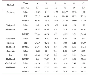
[image:10.595.201.539.441.731.2]We derived these values using 500 simulations for the full information likelih-ood (1), conditional likelihlikelih-ood (6), weighted likelihlikelih-ood (7), calibrated weighted likelihood, complete-data likelihood (12), full-data likelihood (15), and EP like-lihood (20) (see Tables 1-4). We also include the “random approach” based on maximizing the likelihood
Table 1. Relative bias (RBias), relative standard error (RSE) and relative square root mean squared error (RRMSE) of the estimates from various approaches for the parameters in the linear model with BI variation (22). µb=0.2.
Method Value a µx σx µb σb σε
True value 0.5 1.0 5.0 0.2 1.0 0.7
Random RBias −21.09 151.91 59.57 166.77 62.92 1.12
RSE 57.27 46.18 4.36 114.88 12.22 22.28
RRMSE 60.98 158.76 59.73 202.44 64.09 22.29
Weighted RBias 2.62 −0.37 −0.92 1.05 1.28 1.70
likelihood RSE 35.26 40.68 4.70 42.28 5.57 34.06
RRMSE 35.33 40.64 4.79 42.25 5.71 34.06
Calibrated RBias 2.64 −0.40 −0.94 1.37 1.12 2.10
weighted RSE 34.69 40.76 4.71 40.99 5.40 34.09
likelihood RRMSE 34.75 40.72 4.80 40.97 5.51 34.12
Complete RBias −0.63 0.81 0.21 1.86 0.97 8.15
data RSE 42.85 19.48 2.43 25.45 5.11 36.34
likelihood RRMSE 42.81 19.48 2.44 25.49 5.20 37.20
Conditional RBias −4.23 11.83 4.83 15.94 7.46 1.77
likelihood RSE 50.38 32.66 10.30 56.97 16.11 35.53
DOI: 10.4236/ojs.2019.96040 633 Open Journal of Statistics
Continued
Full RBias 0.39 −0.59 −0.28 2.01 0.48 5.38
information RSE 8.19 17.51 2.18 18.55 2.42 15.17
likelihood RRMSE 8.19 17.51 2.20 18.64 2.47 16.09
Full RBias 0.45 −0.80 −0.31 0.53 0.38 6.95
data RSE 8.18 18.46 2.23 17.85 2.38 12.39
likelihood RRMSE 8.18 18.46 2.25 17.84 2.41 14.20
Empirical RBias 0.40 −0.17 −0.07 1.49 0.63 5.89
proportion RSE 8.16 17.60 2.14 17.56 2.36 13.54
[image:11.595.199.537.298.742.2]likelihood RRMSE 8.16 17.58 2.14 17.61 2.44 14.75
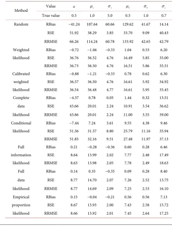
Table 2. Relative bias (RBias), relative standard error (RSE) and relative square root mean squared error (RRMSE) of the estimates from various approaches for the parameters in the linear model with BI variation (22). µb=0.5.
Method Value a µx σx µb σb σε
True value 0.5 1.0 5.0 0.5 1.0 0.7
Random RBias −41.24 107.64 60.66 129.62 41.67 14.14
RSE 51.92 38.29 3.85 33.70 9.09 40.43
RRMSE 66.26 114.24 60.78 133.92 42.65 42.79
Weighted RBias −0.72 −1.06 −0.33 1.04 0.53 6.20
likelihood RSE 36.76 36.52 4.76 16.49 5.85 35.00
RRMSE 36.73 36.50 4.76 16.51 5.86 35.51
Calibrated RBias −0.88 −1.21 −0.33 0.78 0.62 6.30
weighted RSE 36.57 36.50 4.76 16.61 5.92 34.92
likelihood RRMSE 36.54 36.48 4.77 16.61 5.95 35.45
Complete RBias −4.57 0.78 0.05 1.44 0.32 13.51
data RSE 43.66 20.01 2.24 10.91 3.54 36.62
likelihood RRMSE 43.86 20.01 2.24 11.00 3.55 39.00
Conditional RBias −7.44 7.24 3.61 9.55 4.38 9.46
likelihood RSE 51.36 31.37 8.80 25.79 11.16 35.94
RRMSE 51.85 32.16 9.51 27.48 11.97 37.13
Full RBias 0.21 −0.28 −0.36 0.60 0.28 6.46
information RSE 8.64 13.99 2.02 7.77 2.48 17.49
likelihood RRMSE 8.63 13.98 2.05 7.78 2.49 18.63
Full RBias 0.14 0.35 −0.35 0.09 0.28 8.40
data RSE 8.77 14.70 2.07 7.26 2.52 13.75
likelihood RRMSE 8.77 14.69 2.09 7.25 2.53 16.10
Empirical RBias 0.15 −0.04 −0.21 0.56 0.56 7.13
proportion RSE 8.67 13.93 2.00 7.43 2.58 15.72
DOI: 10.4236/ojs.2019.96040 634 Open Journal of Statistics
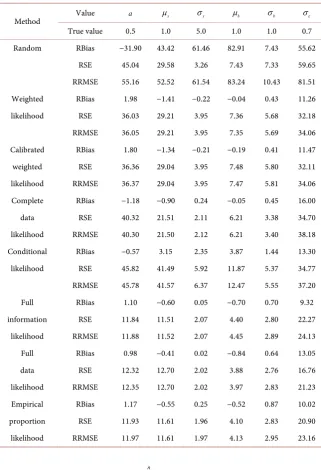
Table 3. Relative bias (RBias), relative standard error (RSE) and relative square root mean squared error (RRMSE) of the estimates from various approaches for the parameters in the linear model with BI variation (22). µb=1.0.
Method Value a µx σx µb σb σε
True value 0.5 1.0 5.0 1.0 1.0 0.7
Random RBias −31.90 43.42 61.46 82.91 7.43 55.62
RSE 45.04 29.58 3.26 7.43 7.33 59.65
RRMSE 55.16 52.52 61.54 83.24 10.43 81.51
Weighted RBias 1.98 −1.41 −0.22 −0.04 0.43 11.26
likelihood RSE 36.03 29.21 3.95 7.36 5.68 32.18
RRMSE 36.05 29.21 3.95 7.35 5.69 34.06
Calibrated RBias 1.80 −1.34 −0.21 −0.19 0.41 11.47
weighted RSE 36.36 29.04 3.95 7.48 5.80 32.11
likelihood RRMSE 36.37 29.04 3.95 7.47 5.81 34.06
Complete RBias −1.18 −0.90 0.24 −0.05 0.45 16.00
data RSE 40.32 21.51 2.11 6.21 3.38 34.70
likelihood RRMSE 40.30 21.50 2.12 6.21 3.40 38.18
Conditional RBias −0.57 3.15 2.35 3.87 1.44 13.30
likelihood RSE 45.82 41.49 5.92 11.87 5.37 34.77
RRMSE 45.78 41.57 6.37 12.47 5.55 37.20
Full RBias 1.10 −0.60 0.05 −0.70 0.70 9.32
information RSE 11.84 11.51 2.07 4.40 2.80 22.27
likelihood RRMSE 11.88 11.52 2.07 4.45 2.89 24.13
Full RBias 0.98 −0.41 0.02 −0.84 0.64 13.05
data RSE 12.32 12.70 2.02 3.88 2.76 16.76
likelihood RRMSE 12.35 12.70 2.02 3.97 2.83 21.23
Empirical RBias 1.17 −0.55 0.25 −0.52 0.87 10.02
proportion RSE 11.93 11.61 1.96 4.10 2.83 20.90
likelihood RRMSE 11.97 11.61 1.97 4.13 2.95 23.16
(
)
1
, |
n
R i i
i
L f y x
=
=
∏
θ (26)as a reference point to see the difference between considering BSS and totally ignoring BSS.
DOI: 10.4236/ojs.2019.96040 635 Open Journal of Statistics
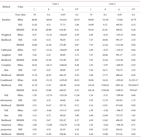
Table 4. Relative bias (RBias), relative standard error (RSE) and relative square root mean squared error (RRMSE) of the estimates from various approaches for the parameters in the VonB model with BI variation (24). Case 1:
(
α β,) (
= 3.643,1.225)
. Case 2:(
α β,) (
= 11.227,0.641)
.Method Value Case 1 Case 2
l∞ k a0 CV l∞ k a0 CV
True value 70 0.2 −0.07 0.2 70 0.2 −0.07 0.2
Random RBias 86.06 −60.83 −614.61 20.35 88.00 −61.04 −23.60 35.79
RSE 15.45 4.31 77.73 3.40 34.09 9.72 495.95 4.13
RRMSE 87.44 60.98 619.49 0.21 94.36 61.81 496.01 0.36
Weighted RBias 9.27 −21.41 −564.69 6.38 2.69 −6.53 −525.27 0.64
likelihood RSE 5.26 6.52 96.69 3.15 7.47 20.66 991.37 2.35
RRMSE 10.66 22.38 572.89 0.07 7.93 21.64 1121.06 0.02
Calibrated RBias 9.27 −21.41 −564.69 6.38 2.69 −6.53 −525.27 0.64
weighted RSE 5.26 6.52 96.69 3.15 7.47 20.66 991.37 2.35
likelihood RRMSE 10.66 22.38 572.89 0.07 7.93 21.64 1121.05 0.02
Complete RBias 10.41 −26.13 −640.04 9.48 1.91 −5.97 −469.93 0.35
data RSE 5.47 6.47 88.99 2.55 5.36 16.71 754.74 2.23
likelihood RRMSE 11.76 26.92 646.19 0.10 5.68 17.73 888.44 0.02
Conditional RBias 12.82 −31.22 −619.49 28.21 30.96 54.24 −659.63 31,525.17
likelihood RSE 31.78 17.67 106.90 14.50 116.24 1536.62 1001.56 703,564.57
RRMSE 34.24 35.86 628.63 0.32 120.18 1536.04 1198.43 7035.67
Full RBias 1.59 −12.76 −523.58 11.26 1.34 −5.51 −399.94 0.60
information RSE 2.92 4.33 64.60 2.44 3.93 11.79 543.65 1.75
likelihood RRMSE 3.32 13.47 527.54 0.12 4.14 13.01 674.48 0.02
Full RBias −2.07 −8.44 −513.17 16.92 1.30 −5.20 −396.57 0.56
data RSE 3.14 4.72 98.26 3.60 4.40 12.60 572.79 1.81
likelihood RRMSE 3.76 9.67 522.47 0.17 4.59 13.62 696.20 0.02
Empirical RBias 1.68 −12.89 −524.59 11.30 1.43 −5.64 −396.78 0.71
proportion RSE 2.92 4.33 65.55 2.45 3.95 11.82 544.41 1.76
likelihood RRMSE 3.37 13.59 528.66 0.12 4.20 13.08 673.22 0.02
in some cases the calibrated WL has a little smaller RRMSEs than WL, and in the other cases the reverse happens, but the differences have no clear pattern, and are too small to draw reliable conclusions. Similarly, even though there is some difference in performance between the complete-data likelihood approach and the two WL approaches, it is not clear which method performs better. The two WL approaches have smaller RRMSEs for a and σε estimation, while the
DOI: 10.4236/ojs.2019.96040 636 Open Journal of Statistics
for µx, σx, µb and σb estimation, its RRMSEs are more than twice of those
from the complete-data likelihood approach. Nevertheless, the conditional like-lihood approach performs substantially better than the random approach.
Simulation results presented in Table 4 provide a comparison of the various estimation approaches for a nonlinear VonB model with BI variation. The out-comes for this nonlinear case are similar to the linear case just described. The full information, full-data and EP likelihood approaches have only tiny differ-ences in performance, and in general perform better than the other approaches. The WL and calibrated WL approaches have almost identical performance. The complete-data likelihood approach has close performance as the two WL ap-proaches and it is not clear which method is better. In Case 1 the conditional li-kelihood approach performs better than the random approach, but worse than all the other approaches including the complete-data approach. In Case 2 its performance is much worse than all the approaches including the random ap-proach. Actually, the conditional likelihood approach failed for this case because it did not converge in 107 of the 500 simulations. All the methods in this study cannot estimate a0 well, with large RBias, large RSEs, and hence large
RRMSEs. In practice we suggest to borrow information from other studies such as larvae studies to fix a0, or equivalently to fix length at age 0, for the VonB
model.
6. Real Data Analysis
The simulation study indicates that the full information likelihood (1), full-data likelihood (15) and EP likelihood (20) approaches perform better than the other estimation methods. In this section we apply these three approaches to fit the VonB model (24) using a dataset collected by DFO in NAFO Division 3N during the spring of 2011. Here we consider only female American plaice because males and females follow different growth models.
The LSAS within each Division involved measuring the length of all fish caught in research trawl tows, classifying them into 2 cm length strata, and sub-sampling a few or no otoliths from each length stratum. The sub-sampling goal in each Division was to obtain about 25 age measurements per 2 cm length stratum by sex if length 10 cm≥ , and about 15 age measurements per stratum without
sex distinguishment if length 10 cm< .
Parameter estimates (ESTs) and the corresponding standard errors (SEs) are provided in Table 5. The three estimation approaches give similar values for all the parameters and SEs, which agrees with their close performance in the simu-lation study. For comparison, we also included estimates from the random ap-proach (26), which result in a substantially larger value for l∞ and a smaller
value for k. The standard errors of the estimates from the random approach are also larger, especially for l∞.
DOI: 10.4236/ojs.2019.96040 637 Open Journal of Statistics
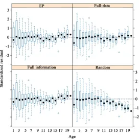
Figure 1. Box-and-whisker plots of standardized residuals vs. age from fitting the VonB model with BI variation (24) to the American plaice data from DFO 2011 Spring survey in NAFO Division 3N by the four likelihood approaches: full information likelihood (Full information), empirical proportion likelihood (EP), full-data likelihood (Full-data) and random sample assumption based likelihood (Random). The black dots are the medians. The boxes indicate the lower and upper quartiles. The ends of the whiskers represent the lowest datum still within 1.5 IQR (interquartile range) of the lower quartile, and the highest datum still within 1.5 IQR of the upper quartile.
Table 5. Parameter estimates (EST) and standard errors (SE) for the VonB model with between-individual variation (24).
Method Value l∞ k a0 CV
Full information EST 61.86 0.10 −0.51 0.11
likelihood SE 1.74 0.0056 0.14 0.0037
EP EST 62.21 0.10 −0.49 0.11
likelihood SE 1.77 0.0056 0.13 0.0037
Full-data EST 65.05 0.093 −0.75 0.11
likelihood SE 1.78 0.0048 0.13 0.0037
Random EST 84.20 0.065 −0.82 0.11
SE 5.53 0.0072 0.17 0.0039
[image:15.595.210.539.489.634.2]young-DOI: 10.4236/ojs.2019.96040 638 Open Journal of Statistics
er ages (≤4) compared to older ages (≥9). The standard deviation (SD) of the standardized residuals at each age is supposed to be 1. However, the calculated SDs (results not shown) transfers from being greater than 1 at younger ages (≤4) to being mainly smaller than about 0.6 at older ages (≥9). These suggest two problems with the model: 1) the BI variation model in (24) under-estimates the variation at shorter lengths and vice-versa at longer lengths for this data, and 2) due to reproduction, the juvenile female American plaice follows a different growth model from the adult female American plaice, which is neglected by the current model.
7. Discussion
We derived the density function (11) for BSS (basic stratified sampling) com-plete data, and constructed the comcom-plete-data likelihood (12), which allows sta-tistical inference when the incomplete data are not well retained. The com-plete-data density can also be used for standardized residual calculation as dis-cussed in Section 3. Residuals are important for validation of fitted models.
Both the complete-data likelihood approach and the random approach make use of only the complete data. The complete approach performs substantially better than the random approach in the simulation studies, indicating the im-portance of correctly incorporating the sampling scheme in the inference me-thods. The conditional likelihood (6) accounts for the sampling scheme ap-proximately by ignoring the randomness in nh in all the strata. Therefore its
performance lies between the random and the complete-data likelihood ap-proaches in almost all the cases in the simulation study. However in some BSS sampling projects where the number of strata is small and the maximum sub-sample size mh for each stratum can usually be obtained, then the conditional
likelihood (6) is appropriate.
Another method to incorporate the sampling scheme is to use the count in-formation of the incomplete data in each stratum, as in the weighted likelihood (WL) and calibrated WL approaches. Even though in the simulation study the two methods of accounting for the sampling scheme, namely the complete-data likelihood and the (calibrated) WL approaches, have comparable performance, the complete-data likelihood requires an appropriate distribution model for co-variates, which can limit its application. The WL and calibrated WL approaches are not subject to this restriction, and hence can be more practical.
DOI: 10.4236/ojs.2019.96040 639 Open Journal of Statistics
On the whole this study indicates that the complete data, the incomplete data, and the sampling scheme are all important for a consistent and efficient statis-tical inference from BSS data.
In this work we found that the EP likelihood approach, which was originally proposed for the variable probability sampling (VPS), works well (or the best together with the full-data and full information likelihood approaches) for BSS data. Its merits will further show up when covariates cannot be modeled effec-tively. This work is under the condition that a valid covariate distribution model is available, which may be a strong assumption in practice. We will explore the case when no appropriate covariate distribution model is available in another paper.
Acknowledgements
Research funding to Nan Zheng was provided by the Ocean Frontier Institute, through an award from the Canada First Research Excellence Fund. Funding was also provided by a Natural Sciences and Engineering Research Council of Canada (NSERC) Discovery grant to NC and NC’s Ocean Choice International Industry Research Chair program at the Marine Institute of Memorial Universi-ty of Newfoundland.
Conflicts of Interest
The authors declare no conflicts of interest regarding the publication of this pa-per.
References
[1] Lawless, J.F., Kalbfleisch, J.D. and Wild, C.J. (1999) Semiparametric Methods for Response-Selective and Missing Data Problems in Regression. Journal of the Royal Statistical Society: Series B (Statistical Methodology), 61, 413-438.
https://doi.org/10.1111/1467-9868.00185
[2] Jewell, N.P. (1985) Least Squares Regression with Data Arising from Stratified Sam-ples of the Dependent Variable. Biometrika, 72, 11-21.
https://doi.org/10.1093/biomet/72.1.11
[3] Rubin, D.B. (1976) Inference and Missing Data. Biometrika, 63, 581-592.
https://doi.org/10.1093/biomet/63.3.581
[4] Cope, J.M. and Punt, A.E. (2007) Admitting Ageing Error When Fitting Growth Curves: An Example Using the Von Bertalanffy Growth Function with Random Ef-fects. Canadian Journal of Fisheries and Aquatic Sciences, 64, 205-218.
https://doi.org/10.1139/f06-179
[5] Cadigan, N.G. and Campana, S.E. (2017) Hierarchical Model-Based Estimation of Population Growth Curves for Redfish (Sebastes mentella and Sebastes fasciatus) off the Eastern Coast of Canada. ICES Journal of Marine Science, 74, 687-697.
https://doi.org/10.1093/icesjms/fsw195
DOI: 10.4236/ojs.2019.96040 640 Open Journal of Statistics
https://doi.org/10.1111/rssc.12340
[7] Carroll, R.J., Ruppert, D., Stefanski, L.A. and Crainiceanu, C.M. (2006) Measure-ment Error in Nonlinear Models: A Modern Perspective. CRC Press, Boca Raton.
https://doi.org/10.1201/9781420010138
[8] Candy, S.G., Constable, A.J., Lamb, T. and Williams, R. (2007) A von Bertalanffy Growth Model for Toothfish at Heard Island Fitted to Length-at-Age Data and Compared to Observed Growth from Mark-Recapture Studies. CCAMLR Science, 14, 43-66.
[9] Scott, A.J. and Wild, C.J. (2011) Fitting Regression Models with Response-Biased Samples. Canadian Journal of Statistics, 39, 519-536.
https://doi.org/10.1002/cjs.10114
[10] Hausman, J.A. and Wise, D.A. (1982) Stratification on Endogenous Variables and Estimation: The Gray Income Maintenance Experiment. In: Manski, C. and McFadden, D., Eds., Structural Analysis of Discrete Data: With Econometric Ap-plications, Chapter 10, MIT Press, Cambridge, 365-391.
[11] Piner, K.R., Lee, H.-H. and Maunder, M.N. (2016) Evaluation of Using Ran-dom-at-Length Observations and an Equilibrium Approximation of the Population Age Structure in Fitting the von Bertalanffy Growth Function. Fisheries Research, 180, 128-137.https://doi.org/10.1016/j.fishres.2015.05.024
[12] Hsieh, D.A., Manski, C.F. and McFadden, D. (1985) Estimation of Response Proba-bilities from Augmented Retrospective Observations. Journal of the American Sta-tistical Association, 80, 651-662.https://doi.org/10.1080/01621459.1985.10478165
[13] Scott, A.J. and Wild, C.J. (1986) Fitting Logistic Models under Case-Control or Choice Based Sampling. Journal of the Royal Statistical Society. Series B ( Methodo-logical), 48, 170-182.https://doi.org/10.1111/j.2517-6161.1986.tb01400.x
[14] Kalbeisch, J.D. and Lawless, J.F. (1988) Estimation of Reliability in Field-Performance Studies. Technometrics, 30, 365-378.
https://doi.org/10.1080/00401706.1988.10488429
[15] Kalbeisch, J.D. and Lawless, J.F. (1988) Likelihood Analysis of Multi-State Models for Disease Incidence and Mortality. Statistics in Medicine, 7, 149-160.
https://doi.org/10.1002/sim.4780070116
[16] Whittemore, A.S. (1997) Multistage Sampling Designs and Estimating Equations.
Journal of the Royal Statistical Society: Series B (Statistical Methodology), 59, 589-602.https://doi.org/10.1111/1467-9868.00084
[17] Breslow, N.E., Lumley, T., Ballantyne, C.M., Chambless, L.E. and Kulich, M. (2009) Improved Horvitz-Thompson Estimation of Model Parameters from Two-Phase Stratified Samples: Applications in Epidemiology. Statistics in Biosciences, 1, 32-49.
https://doi.org/10.1007/s12561-009-9001-6
[18] Saegusa, T. and Wellner, J.A. (2013) Weighted Likelihood Estimation under Two-Phase Sampling. Annals of Statistics, 41, 269.
https://doi.org/10.1214/12-AOS1073
[19] Robins, J.M., Rotnitzky, A. and Zhao, L.P. (1994) Estimation of Regression Coefi-cients When Some Regressors Are Not Always Observed. Journal of the American Statistical Association, 89, 846-866.
https://doi.org/10.1080/01621459.1994.10476818
[20] Thompson, S. (2012) Sampling. John Wiley & Sons, Hoboken.
https://doi.org/10.1002/9781118162934
DOI: 10.4236/ojs.2019.96040 641 Open Journal of Statistics
90, 937-951.https://doi.org/10.1093/biomet/90.4.937
[22] Breslow, N.E. and Cain, K.C. (1988) Logistic Regression for Two-Stage Case-Control Data. Biometrika, 75, 11-20.https://doi.org/10.1093/biomet/75.1.11
[23] Pfeffermann, D. and Sverchkov, M. (1999) Parametric and Semi-Parametric Esti-mation of Regression Models Fitted to Survey Data. Sankhyā: The Indian Journal of Statistics, Series B, 61, 166-186.
[24] Quist, M.C., Pegg, M.A. and DeVries, D.R. (2012) Age and Growth. Fisheries Tech-niques. 3rd Edition, American Fisheries Society, Bethesda, 677-731.
[25] Shelton, A.O., Satterthwaite, W.H., Beakes, M.P., Munch, S.B., Sogard, S.M. and Mangel, M. (2013) Separating Intrinsic and Environmental Contributions to Growth and Their Population Consequences. The American Naturalist, 181, 799-814.https://doi.org/10.1086/670198
[26] Sainsbury, K.J. (1980) Effect of Individual Variability on the von Bertalanffy Growth Equation. Canadian Journal of Fisheries and Aquatic Sciences, 37, 241-247.
https://doi.org/10.1139/f80-031
DOI: 10.4236/ojs.2019.96040 642 Open Journal of Statistics
Appendix: Proof of Theorem 1
Without loss of generality, we assume that
(
y x,)
∈Sh, then(
, | 1;)
Pr(
(
,)
h| 1; Pr , | ,)
(
(
)
h, 1; .)
f y x R= θ = y x ∈S R= θ y x y x ∈S R= θ
Since the selection for full observation is random given
(
y x,)
∈Sh,(
)
(
)
(
(
)
)
(
, |)
Pr , | , h, 1; Pr , | , h; ,
h
f
S R S
Q
∈ = = ∈ = y x
y x y x θ y x y x θ θ
and we have
(
)
(
(
)
)
(
)
(
) (
(
)
)
(
)
0
, |
, | 1; Pr , | 1;
, |
Pr | 1; Pr , | , 1; ,
h
h
h
h m
h h h
n h
f
f R S R
Q f
n R S n R
Q =
= = ∈ =
=
∑
= ∈ =y x y x y x
y x y x θ θ θ θ θ θ (27)
where nh is the sample size in the hth stratum as defined by (4).
(
)
(
)
Pr y x, ∈S n Rh| ,h =1;θ ∝nh, that is, the probability for a selected unit to
be in a stratum h is proportional to the number of vacancies in the stratum h. Also, Pr
(
n Rh| =1;θ)
=Pr(
nh|θ)
, namely, the event {a unit is selected without any further information about its(
y x,)
} is independent of the event {there areh
n units that are selected in the stratum h}.
(
)
dbin(
(
, ,)
,)
if and hence ,Pr |
1 pbin 1, , , if and hence .
h h h h h h
h
h h h h h h
N N Q N m n N
n
m N Q N m n m
< =
= − − ≥ =
θ
Hence, when
(
y x,)
∈Sh,(
)
(
)
(
)
(
)
1
1
, |
, | 1;
dbin , , 1 pbin 1, , ,
h
h
h m
h h h h h h
N
f
f R
Q
N N N Q m m N Q
− = = ∝ × + − −
∑
y xy x θ θ
which can be normalized into (11).
Note that in the case Pr