Active Orientation Models
Georgios Tzimiropoulos, Joan Alabort-i-Medina,
Student Member, IEEE,
Stefanos Zafeiriou
Member, IEEE,
and Maja Pantic
Fellow, IEEE
Abstract—We present Active Orientation Models, generative models of facial shape and appearance, which extend the well-known paradigm of Active Appearance Models (AAMs) for the case of generic face alignment under unconstrained conditions. Robustness stems from the fact that the proposed AOMs employ a statistically robust appearance model based on the principal components of image gradient orientations. We show that when incorporated within standard optimization frameworks for AAM learning and fitting, this kernel PCA results in robust algorithms for model fitting. At the same time, the resulting optimization problems maintain the same computational cost. As a result the main similarity of AOMs with AAMs is computational complexity. In particular, the project-out version of AOMs is as computationally efficient as the standard project-out inverse compositional algorithm which is admittedly one of the fastest algorithms for fitting AAMs. We verify experimentally that (i) AOMs generalize well to unseen variations and (ii) outperform all other state-of-the-art AAM methods considered by a large margin. This performance improvement brings AOMs at least in par with other contemporary methods for face alignment. Finally, we provide Matlab code at http://ibug.doc.ic.ac.uk/resources.
Index Terms—Active Orientation Models, Active Appearance Models, Face alignment.
I. INTRODUCTION
B
ECAUSE of their numerous applications in HCI, face analysis/recognition and medical imaging, the problems of learning and fitting deformable models have been the focus of cutting edge research in computer vision and machine learning for more than two decades. Put in simple terms, these problems can be summarized as follows: Learning a deformable model consists of (a) annotating (typically man-ually) a set of points (or landmarks) over a set of training images capturing an object of interest (e.g. faces), (b) learning a shape model (or point distribution model) which effectively represents the structure and variations among the annotated points and (c) learning appearance models from the image texture associated with the learned shape. Fitting a deformable model utilizes the learned shape and appearance models to detect the location of landmarks in new images; this can be done using regression, classification or could be formulated as a non-linear optimization problem.Depending on the application and/or approach many terms have been used to coin this research: deformable model fitting, Active Shape Models (ASMs) [1], Constrained Local Models (CLMs) [2], [3] landmark localization, point detection, and Active Appearance Models (AAMs) [4], [5] to name a few. The latter approach and the problem of deformable face alignment are of particular interest to this work along with the seminal work [5] for fitting AAMs to face images. AAMs are generative models of shape and appearance typically learned by applying Principal Component Analysis to both shape and
(a) (b)
(c) (d)
Fig. 1. (a) The aim of this work is to detect a set of facial features like the corners of the mouth and the tip of the nose in facial images captured in unconstrained conditions. This problem is known as face alignment in-the-wild. (b) To this end, we propose Active Orientation Models (AOMs), generative deformable models that utilize a statistically robust appearance model based on image gradient orientations. (c) The localization of the facial features is performed in the space of image gradient orientations via a robust algorithm for model fitting and parameter estimation. The obtained fitting result is shown in (d).
texture. In [5], fitting was formulated as a non-linear minimiza-tion problem which consists of minimizing the error between the model instance and the given image with respect to the model parameters which control the shape and appearance variation of faces. This problem was solved using the project-out inverse compositional algorithm, which decouples shape from appearance and results in a computationally efficient algorithm. Owing to its efficiency and accuracy, the algorithm for fitting AAMs proposed in [5] has become the de facto choice for building and fitting person-specific AAMs (i.e. AAMs trained to fit face images of a specific subject which is known in advance).
[image:1.612.335.539.149.387.2]accurately unseen variations, i.e. it is the fitting algorithm which fails to fit the model to unseen images. (b) New tools and insights on how to solve (a) have been recently suggested in [7], [8].
Main results. (a)Models: We propose Active Orientation Model, a generative deformable model that uses a statistically robust appearance model based on the principal components of image gradient orientations (see Fig. 1). We show how to use gradient decent in order to minimize the distance between this non-linear appearance model and a new image with respect to the model parameters. (b)Complexity: Similarly to the AAM formulation of [5], we show that AOMs can be optimized using the project-out inverse compositional algorithm which is admittedly one of the fastest algorithms for fitting deformable models in images. (c) Robustness/Accuracy: To the best of our knowledge, we demonstrate for the first time that this algorithm can be used to fit the learned models to faces not seen in the training set. (d) Comparison to previous work: We conducted a large number of experiments on many popular in-the-wild databases, in which all algorithms were trained, initialized and tested in the same way. We show that the proposed AOM largely outperforms all other state-of-the-art AAM methods considered as well as an enhanced version of a state-of-the-art CLM method [9], and our version of the SDM method of [10]. In the context of our experiments, we also propose a new method: we developed an AAM variant based on least-squares optimization and the appearance model of [11] which is based on similar features. One of the main contributions in our work is to show that the kernel PCA implied by the appearance model of AOMs also outperforms this AAM variant. (d) Code: Similarly to [12], [9], [13], we provide Matlab code at http://ibug.doc.ic.ac.uk/resources.
II. RELATED WORK
A. State-of-the-art.
Because of the inability of AAMs to generalize well to unseen variations, recent research has suggested the use of simpler (often local) and thus easier to optimize models and the application of discriminative methods for model fitting. The family of methods termed ASM-CLMs combine patch-based image representations, discriminatively trained point detectors and global shape constraints to localize landmarks in unseen images [2], [14], [3], [15]. A recent notable example of ASMs is the component-based model of [16] which produces good results on the difficult Helen data set introduced in the same work. Another recent approach that combines the output of SVM-based local detectors with a non-parametric set of global models has been shown to produce excellent results on unconstrained images in [17]. Finally, because sliding-window landmark detectors may be slow, regression-based techniques have been proposed to learn a mapping between local patches and landmarks [17], [12], [18], [19]. Not only do these methods enjoy a high degree of computational efficiency, but also they have been shown to achieve state-of-the-art per-formance for difficult experiments with unconstrained images. In particular, the results presented in the shape regression method of [18] and the supervised decent method of [10] are
impressive and considered state-of-the-art for the difficult data set of LPFW [17]. Finally, a radically different approach to face alignment is the globally optimized part-based model of [13]. Our experiments have shown that [13] is better able to detect faces rather than accurately locating facial landmarks [20].
B. AAMs.
Discriminative methods have been shown to improve the ability of AAMs to fit new faces in [21], [22], [23], [24]. One of the first attempts is the AAM of Cootes and Taylor [11] which is based on regression and features similar to the ones employed by AOMs. Please see [25] for a review on the effect of different texture representations on the performance of regression-based approaches to AAM fitting. Note that no matter the texture representation used, regression methods as proposed in [11] have been reported to produce limited fitting accuracy and robustness (please see [10] for a recent example). One of the main contributions of the proposed work is to illustrate that the kernel PCA implied by the appearance model of AOMs when combined with analytic gradient descent (as opposed to regression) and trained in-the-wild produce results comparable (if not superior) to state-of-the-art methods. Other generic AAMs learn a fitting function through maximizing the score of a two-class classifier (aligned or not aligned) or ranking [21], [22]. Boosting a huge number of Haar features is very inefficient, and results are reported only for low resolution images. This immediately rules out the possibility of accurate landmark localization in high resolution images and it is clearly unsatisfactory. Other discriminative approaches include learning non-linear regressors from features to model param-eters through boosting and simulation [23], [24]. However, all these approaches seem to produce inferior results compared to the family of methods coined CLMs [2], [14], [3], which build upon the Active Shape Model [1]. Finally, a notable example of generative AAMs is the Fourier-Gabor AAMs of [26]. However, as it is mentioned by the authors, Fourier-Gabor AAMs appear to be more suitable for person-specific face alignment for the case of unseen illumination rather than generic face alignment.
III. ACTIVEAPPEARANCEMODELS
A. Shape and appearance models
An AAM is defined by the shape, appearance and motion models. The shape model is typically learned by annotating N fiducial points on the object (e.g. a face) of training image
Ii. These points are said to define the shape of each object.
Next, Procrustes analysis is applied to remove similarity trans-formations from the original shapes. Finally, PCA is applied on the similarity-free shapes si = [x1, y1, x2, y2, . . . xN, yN].
The resulting model {ΦS,0,ΦS ∈ R2N×p} can be used to
represent a test shapesy as
ˆsy =ΦS,0+ΦSp, p=ΦTS(sy−ΦS,0). (1)
The eigenvectors ofΦS represent pose, expression and identity
reference frame defined by the mean shape using the motion model W(x;p) and then applying PCA on the shape-free textures. We choose piecewise affine warps as the motion model in this work. The resulting model{ΦA,0,ΦA∈ RK×q}
can be used to represent a shape-free test texture ay as
ˆ
ay =ΦA,0+ΦAc, c=ΦTA(ay−ΦA,0). (2)
Finally, a model instance is synthesized to represent test object y by warpingayfrom the mean shape¯stoˆsy using piecewise
affine warp.
B. Model fitting
Given a new imageI, inference in AAMs entails estimating
p and c assuming “reasonable” initialization of the fitting process. This initialization is typically performed by placing the mean shape according to the output of an object (in this work, face) detector. Note that only pneeds to be estimated for deformable model fitting. Estimating cis a by-product of the fitting algorithm. Various algorithms and cost functions have been proposed to estimatepandcincluding regression, classification and non-linear optimization methods. The latter approach is of particular interest in this work. It minimizes the `2-norm of the error between the model instance and the
given image with respect to the model parameters as follows
{po,co}= arg min
{p,c}||I[p]−ΦA,0−ΦAc||
2, (3)
where for notational convenience we write I[p](k) to denote the pixel intensity I(W(xk;p)), and I[p] to denote image I(W(x;p)) re-arranged as a K ×1 vector. In a series of seminal papers [27], [5], Baker and Matthews illustrated that problem (3) can be solved using an optimization framework based on the Lukas-Kanade (LK) algorithm [28]. LK algorithm is an image alignment method. Suppose for the time being that an oracle provides co so that c is fixed. Then, (3) becomes
an image alignment problem. In this case, and according to [28], the resulting optimization problem can be solved using Gauss-Newton: First, I[p] is linearized with respect topand then a solution for a ∆p is computed from the set of the derived normal equations obtained by setting the derivative of (3) with respect to ∆p to 0. Finally, p is updated in an additive fashionp←p+ ∆p. We refer the interested reader to [27] for an excellent coverage of the LK algorithm.
Inverse Compositional.As illustrated in [27], [5], problem (3) can be solved in two coordinate frames. The forward case is the standard LK algorithm, as summarized above. In general, forward algorithms are slow because the Jacobian and its inverse must be re-evaluated at each iteration. Fortunately, computationally efficient algorithms can be derived by solving (3) using the inversecompositional framework. Let us dropA
from ΦA for notational convenience and letΦi represent the
i−th column (eigenvector) of Φ. In inverse algorithms, each eigenvector Φi is linearized around p = 0. By additionally
linearizing with respect to c(3) becomes
arg min
∆p,∆c||I[p]−Φ0+J0∆p− m X
i=1
(ci+ ∆ci)(Φi+Ji∆p)||2,
(4)
whereJi is theK×pmatrix each row of which contains the
1×pvector[Φi,x[p](k) Φi,y[p](k)]
∂W(xk;p)
∂p .Φi,x[p](k)and
Φi,y[p](k)are thexandygradients ofΦi for thek−th pixel
and ∂W(xk;p)
∂p ∈ R
2×p is the Jacobian of the piecewise affine
warp. Please see [5] for calculating and implementing ∂∂Wp. All these terms are defined in the model coordinate frame for
p=0 and can be pre-computed. An update for∆cand ∆p
can be obtained in closed form only after second order terms are omitted as follows
arg min
∆p,∆c||I[p]−Φ0−Φc−Φ∆c−J∆p)||
2, (5)
whereJ=J0+P q
i=1ciJi. In [27], the update was derived
as
[∆p; ∆c] =H−s1JTs(I[p]−Φ0−Φc), (6)
whereJs = [Φ;J] ∈ RK×(p+q) and Hs =JTsJs. Once ∆p
is computed, p is updated in a compositional fashion p ← p◦∆p−1, where ◦ denotes the composition of two warps.
(Please see [5] for a principled way of applying the inverse composition to AAMs). This is the well-known simultaneous algorithm.
The simultaneous algorithm is slow because the Jacobian
Js, the Hessian Hs and its inverse must be re-computed at
each iteration. One can easily show that the cost for the Hessian computation is O((p+q)2K). Nonetheless, more efficient ways to optimize (5) exist. Let us define the projection operatorP=E−ΦΦT, whereEis the identity matrix. Then,
a number of works [29], [30], [31] have shown that one can update the appearance and shape parameters in an alternating fashion from
∆c=ΦT(I[p]−Φ0−Φc−J∆p) (7)
∆p=H−a1JTa(I[p]−Φ0), (8)
where the projected-out Jacobian and Hessian are given by
Ja =PJ and Ha = JTaJa, respectively. As shown in [30],
the above update rules result in an algorithm with complexity per iterationO(pqK+p2K+p3)which can be readily handled
by current systems.
By far the most efficient algorithm for fitting AAMs is the so-called project-out inverse compositional algorithm, which in essence is a LK algorithm. This algorithm decouples shape and appearance by solving (5) in the subspace orthogonal to
Φ. Observe that||I[p]−Φ0−Φc||2
P=||I[p]−Φ0|| 2 P
1. Hence
an update for∆pcan be computed by optimizing
arg min
∆p ||I[p]−Φ0−J0∆p)|| 2
P. (9)
The solution to the above problem is given by
∆p=H−p1JTp(I[p]−Φ0), (10)
where the projected-out Jacobian Jp = PJ0 and Hessian Hp = JTpJp, can be both pre-computed. This reduces the
cost per iteration toO(pK), only [5], which is the cost of the inverse compositional LK algorithm [27]. This algorithm has been shown to track faces at 300 fps [6].
1For a vectorx, we use the notation||x||2
P to denote the weighted norm
IV. ACTIVEORIENTATIONMODELS
The deformable model fitting framework of the previous section and especially the project-out inverse compositional algorithm has been highly criticized as difficult to optimize mainly due to the high-dimensional parameter space and the existence of numerous undesirable local minima in the derived cost functions. Therefore, the problem in hand is how to avoid these local minima during optimization. We propose to address this problem by using a kernel PCA based on a similarity criterion robust to outliers. In particular, AOMs employ a statistically robust appearance model based on the principal components of images gradient orientations. As we show below both shape and texture models can be optimized in a standard least-squares framework which results in com-putationally efficient algorithms.
A. Appearance Model
At the heart of the appearance model of AOMs there exists a robust kernel for measuring similarity. We define outliers to be anything that the learned appearance model cannot reconstruct because (a) it was not seen in the training set (e.g. appearance variation due to different identity, expression or illumination) (b) it does not belong to the face space at all (e.g. glasses) and (c) it was excluded fromΦAas noise because in any case the
number of principal components inΦAshould be kept as small
as possible so that the model is easier to optimize and cannot generate appearance which is unrelated to faces. Note that as it was shown in [6] for some cases of interest (e.g. appearance variation in frontal views), a very compact appearance space, learned from a training set with a few persons only, in general, results in relatively small reconstruction errors of unseen faces. This illustrates that a generative model is not an unreasonable choice for generic deformable model fitting. All that is needed is a robust cost function to fit this model.
A general framework for robust estimation is weighted least squares [32]. Let us definee=I[p]−¯a−ΦAc. Then, weighted
least squares methods optimize
{po,co}= arg min
{p,c}e
TQe,
(11)
where Q ∈ R{K,K} is a diagonal weighting matrix which down-weighs pixels corrupted by outliers. An ideal case would beQk = 0if pixelkis an outlier andQk = 1otherwise. The
estimation ofQalong with the optimal model parameters have been extensively studied in the literature of robust statistics (please see [32] for a review). However, none of these out-of-the-box approaches has been proven successful so far in AAM fitting because (a) the noise model for outliers in our case is very hard to define and (b) the estimation process is also very prone to local minima.
We propose to address this problem in AAMs by using a robust similarity criterion based on image gradient orientations [7], [8]. Suppose that we wish to measure the similarity between two images Ii,i= 1,2. For each image, we extract
image gradients gi,x,gi,y and the corresponding estimates of
gradient orientation φi. Let us denote byzi the the so-called
normalized gradients
zi=
1
√
K[cos(φi)
T, sin(φ
i) T]T,
(12)
wherecos(φi) = [cos(φi(1)), . . . ,cos(φi(K))]T andsin(φ i)
is similarly defined. Then, the following kernel can be used to measure image similarity
s = zT1z2
= 1
K
X
k∈Ω
cos(φ1(k)−φ2(k)), (13)
whereΩdenotes the image support.
Let us also denote byΩ1 the image support that is
outlier-free and Ω2 the image support that is corrupted by outliers
(Ω = Ω1∪Ω2). Then, as it was shown in [8], under some
assumptions, it holds
X
k∈Ω2
cos(φ1(k)−φ2(k))≈0. (14)
Note that (a) in contrary to [27], no assumption about the structure of outliers is made and (b) no actual knowledge of Ωis required. Based on (14), we can re-write (13) as follows
s = X
k∈Ω1
cos(φ1(k)−φ2(k)) + X
k∈Ω2
cos(φ1(k)−φ2(k))
= X
k∈Ω1
1·cos(φ1(k)−φ2(k)) + X
k∈Ω2
·cos(φ1(k)−φ2(k))
≈ zT1Qidealz2, (15)
where→0andQidealis the “ideal” weighting matrix defined
above. Note that Qideal in (15) is never calculated explicitly.
We can write (15) only because outliers are approximately “canceled out” when the above kernel is used to measure image similarity.
The robust kernel of (13) can be used to define a kernel PCA [8]. The appearance model in AOMs is learned using this robust PCA. Note that the kernel can be written using the explicit mapping of (12) and therefore no pre-image computation is required. Suppose that for each training image
Ii,i= 1, . . . hwe extract the shape-free normalized gradients
of each training face zi, and then we form the data matrix Z∈ R2K×h the columns of which containz
i. Then we apply
PCA onZ. We denote by
ΦZ= [Φx;Φy]∈ <2K×q (16)
the learned appearance model, where Φx andΦy ∈ <K×q
are the parts corresponding to the cosine and sine terms, respectively. Note that to preserve the kernel properties no subtraction of the “mean” normalized gradient is needed and the first eigenvector is treated as the mean where it is required.
B. Shape Model
C. Inference
We perform inference in AOMs by minimizing the error between a test image and a model instance
{po,co}= arg max
{p,c}||z[p]−ΦZc||
2, (17)
where z[p](k) denotes the normalized gradient of
I(W(xk;p)). Our optimization strategies are summarized
below:
Simultaneous.The simultaneous AOM minimizes (17) with respect to both {p,c}. This requires the computation of the Hessian (O((p+q)22K)) and its inverse (O((p+q)3)) and is
very slow. For this reason, we did not look into this algorithm further.
Alternating. The minimization of (17) can be also per-formed in an alternating fashion. Because the “mean” nor-malized gradient is the first eigenvector of our kernel PCA, we write
J=
q X
i=0
ciJiJi= [Ji,x;Ji,y], (18)
where Ji,x and Ji,y are the Jacobians computed from Φi,xandΦi,y respectively. As before let us drop the
depen-dency of notation from Z and define the projection operator P=E−ΦΦT. Let us also define the projected-out Jacobian and Hessian
Ja=PJHa=JTaJa. (19)
Then, the updates for the appearance and shape parameters are given by
∆c=ΦT(z[p]−Φc−J∆p) (20)
∆p=H−a1JTaz[p]. (21)
For completeness, we derive the update rules for∆cand∆p
in the Appendix. Notice that in the above update for∆p, the “error image” is implicitly calculated because
JTaz[p] =JTPTz[p] =JT(z[p]−Φc), (22)
which shows that the error is simply the difference between the normalized gradient and its reconstruction from the appearance subspace. The steps of the algorithm are summarized in Algorithm 1.
Algorithm 1 AOM - Alternating Optimization
Given:Models{ΦS,0,ΦS}andΦZ, and current estimates for candp
Pre-compute: JacobianJi for each appearance eigenvector
1: repeat
2: Compute warped image I[p] and extract normalized gradientsz[p]
3: CalculateJ andJa from (18) and (19)
4: CalculateHa andH−a1 from (19)
5: Calculate∆cand∆pfrom (20) and (21) 6: Update fromc←c+ ∆candp←p◦∆p−1
7: untilconvergence
The main cost of the above algorithm is in steps 3-5. In
particular, the complexity of calculatingJandJa isO(q2K)
andO(pq2K), respectively. The complexity of calculatingHa
andH−1
a is O(p22K)and O(p3). Finally, the complexity of
calculating∆cand∆pisO(q2K)andO(p2K).
Project-out. To derive the project-out AOM fitting algo-rithm we treat the first eigenvectorΦ0 as the “mean
normal-ized gradient”, and then perform a first order Taylor on it
Φ0=Φ0[0] +J0∆p. Then, we write
||z[p]−Φ0−J0∆p||2P=||z[p]−J0∆p||2P, (23)
and hence the update for∆pcan be readily derived as
∆p=H−p1JTpz[p], (24)
where ,
Jp=PJ0,Hp=JTpJp (25)
can be both pre-computed. Overall, the steps of the algorithm are summarized in Algorithm 2.
Algorithm 2 AOM - Project-Out
Given:Models{ΦS,0,ΦS}andΦZ, and current estimates for candp
Pre-compute:R=H−1
p JTp from (25)
1: repeat
2: Compute warped image I[p] and extract normalized gradientsz[p]
3: Calculate ∆p=Rz[p] 4: Update from p←p◦∆p−1
5: untilconvergence
The main cost of the above algorithm is in step 2. In particular, calculating∆ptakesO(q2K)only, and hence this algorithm is extremely fast.
V. RESULTS
Evaluating and comparing different methods for deformable object and face alignment is difficult, because when training and fitting codes are not publicly available, various implemen-tation aspects including training and initialization can be very different, and this in turn possibly results in very different performance. Hence, for the sake of a fair comparison, in our experiments we did not attempt to directly compare our results with the ones reported in previously published methods. Instead, the main focus of our experiments was to compare the proposed AOMs with methods for which we have in-house implementations and hence comparison is fairer. In particular, we compare AOMs with: (a) an AAM based on pixel intensities (PI) [30], (b) a state-of-the-art Gabor-Fourier (GF) AAM [26], (c) an AAM using the edge structure gradient features of [11] (ES), (d) the CLM method of [9] using discriminatively trained HOG features for local detectors2and (e) our version of the SDM method of [10]. Both CLM and SDM are trained on the same data as our AAMs. All variants of AAMs were fitted using both alternating and project-out
inverse compositional algorithms implemented in a multi-scale (pyramid) fashion with 15 shape parameters at the highest level. Note that the the edge structure gradient features of [11] are similar to the normalized gradients of AOMs, with the main difference being that [11] uses the gradient magnitude to normalize the gradients which is less robust to outliers [7]. We further note that these features have been employed only in regression-based approaches to AAM fitting, and hence their combination with non-linear optimization (alternating or project-out) is a method that is also proposed for the first time (to the best of our knowledge) in this work. Similarly to our previous work [7], we evaluate these features because they are similar to the normalized gradients of the appearance model of AOMs.
For our experiments we used the training set of LFPW [17] to train all aforementioned methods. For testing, we used the test set of LFPW, as well as the test set of Helen [16] and AFW [13]. Although all databases are in-the-wild, LPFW mainly contain images of celebrities with posed smiles while the faces of Helen and AFW seem to be much more natural, with much more shape and appearance variation, and hence are even more challenging to fit. For all databases, we used the landmark annotations of the 300-W challenge [33], [34]. In order to assess performance, we used the same average (computed over all 68 points) point-to-point Euclidean error normalized by the face size as the one used in [13]. Similarly to [13], for this error measure, we produced the cumulative curve corresponding to the percentage of test images for which the error was less than a specific value. In all cases, fitting was initialized by the bounding box of the detector proposed in [13].
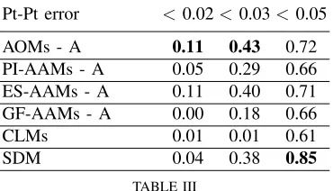
Our comparisons/results are summarized in Fig. 2 and Ta-bles 1-6. The quality of fittings produced by AOM alternating and project-out optimization can be visually compared in Fig. 3. As we may observe, AOM alternating optimization produces better fitting results especially with regards to the face boundary. Additional fitting results obtained with AOM alternating optimization and SDM on selected challenging images from the AFW database can be seen in Fig. 4. Each row of Fig. 4 highlights a different source of facial variation: age, pose, illumination, expression, occlusion and low resolution or blur. Overall, AOMs are able to fit some difficult cases of faces from Helen and AFW data sets with shape and appearance variation quite different from that seen during training on LPFW. From the presented results we conclude the following: Alternating optimization.(a) AOM alternating optimization algorithm performs the best among all algorithms, with ES-AAMs achieving similar performance. (b) All ES-AAMs when trained in-the-wild and optimized using alternating optimiza-tion perform notably well. These results are not so surprising and should be attributed to the appearance model of the AAM which for all variants was trained in-the-wild. We refer the reader to [30] for a detailed discussion. (c) All AAMs when trained in-the-wild and optimized using alternating optimiza-tion largely outperform the state-of-the-art CLM method. (d) For errors greater than 0.05, SDM is the most robust method. Project-out.(a) AOM project-out is by far the most robust project-out algorithm, outperforming both ES-AAMs and GF-AAMs. Notably, its fitting accuracy is similar to that of
PI-Pt-Pt error <0.02 <0.03 <0.05
AOMs - A 0.33 0.78 0.93 PI-AAMs - A 0.2 0.62 0.91 ES-AAMs - A 0.35 0.74 0.92 GF-AAMs - A 0.10 0.56 0.84
CLMs 0.00 0.05 0.80
SDM 0.14 0.67 0.98
TABLE I
FITTING PERFORMANCE ONLPFWUSING ALTERNATING OPTIMIZATION:
PROPORTION OF IMAGES THAT WERE FITTED WITHPT-PT ERROR<0.02,
<0.03AND<0.05.
Pt-Pt error <0.02<0.03<0.05
AOMs - A 0.21 0.66 0.88 PI-AAMs - A 0.10 0.50 0.82 ES-AAMs - A 0.20 0.66 0.87 GF-AAMs - A 0.02 0.37 0.84 CLMs 0.00 0.04 0.74 SDM 0.05 0.49 0.94
TABLE II
FITTING PERFORMANCE ONHELENUSING ALTERNATING OPTIMIZATION:
PROPORTION OF IMAGES THAT WERE FITTED WITHPT-PT ERROR<0.02,
<0.03AND<0.05.
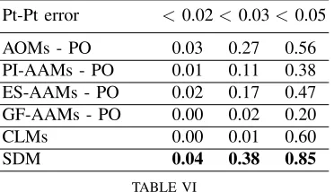
AAM when optimized using alternating optimization. This is a notable result given that AOM project-out is significantly faster. These results also clearly illustrate the robustness of the proposed AOM: the project-out algorithm is literally a LK algorithm the goal of which is to align the test image with the mean image of the appearance subspace. Because the appearance model is not employed to compensate for large discrepancies in appearance between the test image and the mean (as opposed to alternating optimization), a robust algorithm is required to perform the alignment. As the presented results clearly illustrate, AOM project-out is the most robust alignment algorithm. We note that these results are in accordance with the ones presented in our previous work [7] which have shown that the kernel of AOMs performs by far the best for LK-based image-to-image alignment. (b) AOM project-out largely outperforms the state-of-the-art CLM method. This is an important result because AOM project-out is also faster than the CLM method which relies on filtering the image with HOG filters.
Cross-database experiments. As expected, for these ex-periments performance drops for all methods but the rela-tive difference in performance is the similar. Again, AOM outperforms all other algorithms considered. The drop in performance should be also attributed to the less accurate initialization provided by the face detector.
VI. CONCLUSIONS
Fig. 2. Fitting performance on LPFW (first row), HELEN (second row) and AFW (third row). Left column: Alternating optimization. Right column: Project-out optimization. In all figures the point-to-point error normalized by the face size vs the percentage of test images is plotted.
Pt-Pt error <0.02<0.03<0.05
AOMs - A 0.11 0.43 0.72 PI-AAMs - A 0.05 0.29 0.66 ES-AAMs - A 0.11 0.40 0.71 GF-AAMs - A 0.00 0.18 0.66 CLMs 0.01 0.01 0.61 SDM 0.04 0.38 0.85
TABLE III
FITTING PERFORMANCE ONAFWUSING ALTERNATING OPTIMIZATION:
PROPORTION OF IMAGES THAT WERE FITTED WITHPT-PT ERROR<0.02,
<0.03AND<0.05.
Pt-Pt error <0.02<0.03<0.05
AOMs - PO 0.17 0.47 0.81 PI-AAMs - PO 0.08 0.28 0.61 ES-AAMs - PO 0.10 0.39 0.71 GF-AAMs - PO 0.00 0.09 0.45 CLMs 0.00 0.05 0.79 SDM 0.14 0.67 0.98
TABLE IV
FITTING PERFORMANCE ONLPFWUSING PROJECT-OUT ALGORITHM:
PROPORTION OF IMAGES THAT WERE FITTED WITHPT-PT ERROR<0.02,
Fig. 3. Comparison between AOM Alternating and Project-Out Optimization on HELEN. Odd rows: Alternating optimization. Even rows: project-out optimization. Although our system was trained on LPFW which primarily contains celebrity faces with posed smiles, it is able to fit some difficult faces from Helen with shape and appearance variation quite different from the faces of LPFW. Alternating optimization fits the face boundary better.
Pt-Pt error <0.02<0.03<0.05
AOMs - PO 0.12 0.41 0.72 PI-AAMs - PO 0.05 0.20 0.49 ES-AAMs - PO 0.07 0.31 0.61 GF-AAMs - PO 0.00 0.07 0.40 CLMs 0.00 0.04 0.74 SDM 0.05 0.49 0.94
TABLE V
FITTING PERFORMANCE ONHELENUSING PROJECT-OUT ALGORITHM:
PROPORTION OF IMAGES THAT WERE FITTED WITHPT-PT ERROR<0.02,
<0.03AND<0.05.
Pt-Pt error <0.02<0.03<0.05
AOMs - PO 0.03 0.27 0.56 PI-AAMs - PO 0.01 0.11 0.38 ES-AAMs - PO 0.02 0.17 0.47 GF-AAMs - PO 0.00 0.02 0.20 CLMs 0.00 0.01 0.60 SDM 0.04 0.38 0.85
TABLE VI
FITTING PERFORMANCE ONAFWUSING PROJECT-OUT ALGORITHM:
PROPORTION OF IMAGES THAT WERE FITTED WITHPT-PT ERROR<0.02,
<0.03AND<0.05.
gradient orientations. We demonstrated that when incorporated within standard optimization frameworks for AAM learning and fitting, this kernel PCA results in robust and efficient algorithms for model fitting. Finally, we showed that the proposed AOM largely outperforms all other state-of-the-art AAM methods considered as well as a state-of-the-art CLM method, when all methods are trained on the same training set and initialized in the same way. Future work includes combining AOMs with the Gauss-Newton Deformable Part
Model which by-passes the complicated motion model of AAMs [35].
ACKNOWLEDGMENT
This work is funded in part by the European Community 7th Framework Programme [FP7/2007-2013] under grant agree-ment no. 611153 (TERESA). The work of Joan Alabort-i-Medina is funded by DTA studentship from Imperial College London and by the Qualcomm Innovation Fellowship. The work by Stefanos Zafeiriou is funded in part by the EPSRC project EP/J017787/1 (4DFAB).
APPENDIX
In this section we will derive (20) and (21). After lineariza-tion of (17), we obtain the following optimizalineariza-tion problem
arg min
∆p,∆c||z[p]−ΦZc−Φ∆c−J∆p)|| 2.
(26)
To solve the above problem our strategy is to optimize (26) first with respect to ∆c, and then plug in the solution back to (26). Then, we can optimize (26) with respect to ∆p. In particular, let us denote byC1=z[p]−Φ∆c−J∆p. Then,
we have
arg min
∆c(C1−ΦZc)
T(C
1−Φc). (27)
By setting the derivative of the above with respect to ∆c to
0, we readily obtain (20)
∆c=ΦTZC1=ΦTZ(z[p]−Φ∆c−J∆p). (28)
Plugging the above to (26) and, after some straightforward mathematical manipulations, we get the following optimiza-tion problem for∆p
arg min
∆p(z[p]−J∆p)
TP(z[p]−J∆p), (29)
whereP=E−ΦZΦTZ. By setting the derivative of the above
Fig. 4. Fitting results obtained with our method and SDM on selected images from the AFW database. Different rows highlight a different source of facial variation: age, pose, illumination, expression, occlusion and low resolution or blur. Odd rows: AOMs. Even rows: SDM
REFERENCES
[1] T.F. Cootes, C.J. Taylor, D.H. Cooper, and J. Graham, “Active shape models-their training and application,”CVIU, vol. 61, no. 1, pp. 38–59,
1995.
3054–3067, 2008.
[3] J.M. Saragih, S. Lucey, and J.F. Cohn, “Face alignment through subspace constrained mean-shifts,” inICCV, 2009.
[4] T.F. Cootes, G.J. Edwards, and C.J. Taylor, “Active appearance models,”
TPAMI, vol. 23, no. 6, pp. 681–685, 2001.
[5] I. Matthews and S. Baker, “Active appearance models revisited,”IJCV, vol. 60, no. 2, pp. 135–164, 2004.
[6] R. Gross, I. Matthews, and S. Baker, “Generic vs. person specific active appearance models,”Image and Vision Computing, vol. 23, no. 12, pp. 1080–1093, 2005.
[7] G. Tzimiropoulos, S. Zafeiriou, and M. Pantic, “Robust and efficient parametric face alignment,” inICCV, 2011.
[8] G. Tzimiropoulos, S. Zafeiriou, and M. Pantic, “Subspace learning from image gradient orientations,” IEEE TPAMI, vol. 34, no. 12, pp. 2454– 2466, 2012.
[9] J.M. Saragih, S. Lucey, and J.F. Cohn, “Deformable model fitting by regularized landmark mean-shift,” IJCV, vol. 91, no. 2, pp. 200–215, 2011.
[10] Xuehan Xiong and Fernando De la Torre, “Supervised descent method and its applications to face alignment,” 2013.
[11] T.F. Cootes and C.J. Taylor, “On representing edge structure for model matching,” inCVPR, 2001.
[12] M. Valstar, B. Martinez, X. Binefa, and M. Pantic, “Facial point detection using boosted regression and graph models,” inCVPR, 2010. [13] X. Zhu, , and D. Ramanan, “Face detection, pose estimation, and
landmark estimation in the wild.,” inCVPR, 2012.
[14] S. Lucey, Y. Wang, M. Cox, S. Sridharan, and J.F. Cohn, “Efficient constrained local model fitting for non-rigid face alignment,” Image and Vision Computing, vol. 27, no. 12, pp. 1804–1813, 2009. [15] Pedro Martins, Rui Caseiro, Jo˜ao F Henriques, and Jorge Batista,
“Discriminative bayesian active shape models,” inECCV. 2012. [16] Vuong Le, Jonathan Brandt, Zhe Lin, Lubomir Bourdev, and Thomas S
Huang, “Interactive facial feature localization,” inECCV. 2012. [17] P.N. Belhumeur, D.W. Jacobs, D.J. Kriegman, and N. Kumar,
“Local-izing parts of faces using a consensus of exemplars,” inCVPR, 2011. [18] Xudong Cao, Yichen Wei, Fang Wen, and Jian Sun, “Face alignment
by explicit shape regression,” inCVPR, 2012.
[19] Tim F Cootes, Mircea C Ionita, Claudia Lindner, and Patrick Sauer, “Robust and accurate shape model fitting using random forest regression voting,” inECCV. 2012.
[20] Georgios Tzimiropoulos, Joan Alabort-i Medina, Stefanos Zafeiriou, and Maja Pantic, “Generic active appearance models revisited,” inACCV 2012, 2013.
[21] X. Liu, “Generic face alignment using boosted appearance model,” in
CVPR, 2007.
[22] H. Wu, X. Liu, and G. Doretto, “Face alignment via boosted ranking model,” inCVPR, 2008.
[23] J. Saragih and R. Gocke, “Learning aam fitting through simulation,”
Pattern Recognition, vol. 42, no. 11, pp. 2628–2636, 2009.
[24] J. Saragih and R. Goecke, “A nonlinear discriminative approach to aam fitting,” inICCV, 2007.
[25] P Kittipanya-ngam and TF Cootes, “The effect of texture representations on aam performance,” inICPR, 2006.
[26] R. Navarathna, S. Sridharan, and S. Lucey, “Fourier active appearance models,” inICCV, 2011.
[27] S. Baker, R. Gross, and I. Matthews, “Lucas-kanade 20 years on: Part 3,”Robotics Institute, Carnegie Mellon University, Tech. Rep. CMU-RI-TR-03-35, 2003.
[28] Bruce D Lucas, Takeo Kanade, et al., “An iterative image registration technique with an application to stereo vision,” inProceedings of the 7th international joint conference on Artificial intelligence, 1981. [29] Gregory D Hager and Peter N Belhumeur, “Efficient region tracking
with parametric models of geometry and illumination,” IEEE TPAMI, vol. 20, no. 10, pp. 1025–1039, 1998.
[30] Georgios Tzimiropoulos and Maja Pantic, “Optimization problems for fast aam fitting in-the-wild,” inICCV, 2013.
[31] George Papandreou and Petros Maragos, “Adaptive and constrained algorithms for inverse compositional active appearance model fitting,” inCVPR. IEEE, 2008.
[32] F. De La Torre and M.J. Black, “A framework for robust subspace learning,”IJCV, vol. 54, no. 1, pp. 117–142, 2003.
[33] Christos Sagonas, Georgios Tzimiropoulos, Stefanos Zafeiriou, and Maja Pantic, “A semi-automatic methodology for facial landmark annotation,” inCVPR-W, 2013.
[34] Christos Sagonas, Georgios Tzimiropoulos, Stefanos Zafeiriou, and Maja Pantic, “300 faces in-the-wild challenge: The first facial landmark
localization challenge,” inComputer Vision Workshops (ICCVW), 2013 IEEE International Conference on. IEEE, 2013.
Georgios Tzimiropoulos Georgios Tzimiropoulos received the diploma degree in Electrical and Com-puter Engineering from Aristotle University of Thes-saloniki, Greece, and the M.Sc. and Ph.D. degrees in Signal Processing and Computer Vision both from Imperial College London, UK. He is currently a Se-nior Lecturer (Assistant Professor) with the School of Computer Science at the University of Lincoln, UK. After the completion of his Ph.D., he worked as a Research and Development engineer with Imperial College/Selex Galileo. From 2010 to 2012, he was a Research Associate in the Department of Computing at Imperial College working on face analysis. He is currently an Associate Editor of the Image and Vision Computing Journal. His main research interests are in the areas of face and object recognition, alignment and tracking and facial expression analysis.
Joan Alabort-i-Medina received a BSc degree in Computer Science and Engineering from Universitat Autnoma de Barcelona in 2008 and a MSc degree in Visual Information Processing from Imperial Col-lege London in 2011. He is currently working to-wards a PhD degree in Computer Vision at Imperial College London. His research interests lie in the fields of Computer Vision, Machine Learning and Human-Computer Interaction.
Stefanos Zafeiriou (M’09), is a Lecturer (equiv-alent to Assistant Professor) in Pattern Recogni-tion/Statistical Machine Learning for Computer Vi-sion in the Department of Computing, Imperial College London. He has been awarded one of the prestigious Junior Research Fellowships (JRF) from Imperial College London in 2011 to start his own independent research group. He has received various awards during his doctoral and postdoctoral studies. Dr. Zafeiriou currently serves as an Associate Editor in IEEE Transactions on Cybernetics and Image and Vision Computing journal. He has been guest editor in more than five journal special issues and co-organized more than five workshops/ special sessions in top venues such as CVPR/FG/ICCV/ECCV. He has co-authored more than 40 journal papers mainly on novel statistical machine learning methodologies applied to computer vision problems such as 2D/3D face analysis, deformable object fitting and tracking, shape from shading, human behaviour analysis etc published in the most prestigious journals in his field of research (such as IEEE T-PAMI, IJCV, IEEE T-IP, IEEE T-NNLS, IEEE T-VCG, IEEE T-IFS etc), as well many papers in top conferences (such as CVPR, ICCV, ECCV, ICML etc). His students are frequent recipients of very prestigious and highly competitive fellowships such as Google Fellowship, Intel Fellowship and the Qualcomm fellowship.