Hans Petter Langtangen
Python Scripting
for Computational
Science
Third Edition
With 62 Figures
Simula Research Laboratory Martin Linges vei 17, Fornebu P.O. Box 134
1325 Lysaker, Norway [email protected]
On leave from:
Department of Informatics University of Oslo
P.O. Box 1080 Blindern 0316 Oslo, Norway http://folk.uio.no/hpl
The author of this book has received financial support from the NFF – Norsk faglitterær forfatter- og oversetterforening.
ISBN 978-3-540-73915-9 e-ISBN 978-3-540-73916-6
DOI 10.1007/978-3-540-73916-6
Texts in Computational Science and Engineering ISSN 1611-0994
Library of Congress Control Number: 2007940499
Mathematics Subject Classification (2000): 65Y99, 68N01, 68N15, 68N19, 68N30, 97U50, 97U70
© 2008, 2006, 2004 Springer-Verlag Berlin Heidelberg
This work is subject to copyright. All rights are reserved, whether the whole or part of the material is concerned, specifically the rights of translation, reprinting, reuse of illustrations, recitation, broad-casting, reproduction on microfilm or in any other way, and storage in data banks. Duplication of this publication or parts thereof is permitted only under the provisions of the German Copyright Law of September 9, 1965, in its current version, and permission for use must always be obtained from Springer. Violations are liable to prosecution under the German Copyright Law.
The use of general descriptive names, registered names, trademarks, etc. in this publication does not imply, even in the absence of a specific statement, that such names are exempt from the relevant protective laws and regulations and therefore free for general use.
Typesetting: by the author using a Springer TEX macro package Cover design: WMX Design GmbH, Heidelberg
Production: LE-TEX Jelonek, Schmidt & Vöckler GbR, Leipzig Printed on acid-free paper
9 8 7 6 5 4 3 2 1
Preface to the Third Edition
Numerous readers of the second edition have notified me about misprints and possible improvements of the text and the associated computer codes. The resulting modifications have been incorporated in this new edition and its accompanying software.
The major change between the second and third editions, however, is caused by the new implementation of Numerical Python, now callednumpy. The new numpy package encourages a slightly different syntax compared to the old Numeric implementation, which was used in the previous editions. Since Numerical Python functionality appears in a lot of places in the book, there are hence a huge number of updates to the new suggestednumpysyntax, especially in Chapters 4, 9, and 10.
The second edition was based on Python version 2.3, while the third edition contains updates for version 2.5. Recent Python features, such as generator expressions (Chapter 8.9.4), Ctypes for interfacing shared libraries in C (Chapter 5.2.2), thewithstatement (Chapter 3.1.4), and thesubprocess module for running external processes (Chapter 3.1.3) have been exemplified to make the reader aware of new tools. Regarding Chapter 3.1.3,os.system is not used in the book anymore, instead we recommend the commands or subprocess modules.
Chapter 4.4.4 is new and gives a taste of symbolic mathematics in Python. Chapters 5 and 10 have been extended with new material. For example, F2PY and the Instant tool are very convenient for interfacing C code, and this topic is treated in detail in Chapters 5.2.2, 10.1.1, and 10.1.2 in the new edition. Installation of Python itself and the many add-on modules have become increasingly simpler over the years withsetup.py scripts, which has made it natural to simplify the descriptions in Appendix A.
Thepy4cspackage with software tools associated with this book has un-dergone a major revision and extension, and the package is now maintained under the namescitools and distributed separately. The namepy4csis still offered as a nickname forscitoolsto make old scripts work. The newscitools package is backward compatible withpy4csfrom the second edition.
Several people has helped me with preparing the new edition. In par-ticular, the substantial efforts of Pearu Peterson, Ilmar Wilbers, Johannes H. Ring, and Rolv E. Bredesen are highly appreciated.
The Springer staff has, as always, been a great pleasure to work with. Special thanks go to Martin Peters, Thanh-Ha Le Thi, and Andrea K¨ohler for their extensive help with this and other book projects.
The second edition features new material, reorganization of text, improved examples and software tools, updated information, and correction of errors. This is mainly the result of numerous eager readers around the world who have detected misprints, tested program examples, and suggested alternative ways of doing things. I am greatful to everyone who has sent emails and contributed with improvements. The most important changes in the second edition are briefly listed below.
Already in the introductory examples in Chapter 2 the reader now gets a glimpse of Numerical Python arrays, interactive computing with the IPython shell, debugging scripts with the aid of IPython and Pdb, and turning “flat” scripts into reusable modules (Chapters 2.2.5, 2.2.6, and 2.5.3 are added). Several parts of Chapter 4 on numerical computing have been extended (es-pecially Chapters 4.3.5, 4.3.6, 4.3.7, and 4.4). Many smaller changes have been implemented in Chapter 8; the larger ones concern exemplifying Tar archives instead of ZIP archives in Chapter 8.3.4, rewriting of the mate-rial on generators in Chapter 8.9.4, and an example in Chapter 8.6.13 on adding new methods to a class without touching the original source code and without changing the class name. Revised and additional tips on opti-mizing Python code have been included in Chapter 8.10.3, while the new Chapter 8.10.4 contains a case study on the efficiency of various implemen-tations of a matrix-vector product. To optimize Python code, we now also introduce the Psyco and Weave tools (see Chapters 8.10.4, 9.1, 10.1.3, and 10.4.1). To reduce complexity of the principal software example in Chapters 9 and 10, I have removed evaluation of string formulas. Instead, one can use the revisedStringFunction tool from Chapter 12.2.1 (the text and software regarding this tool have been completely rewritten). Appendix B.5 has been totally rewritten: now I introduce Subversion instead of CVS, which results in simpler recipes and shorter text. Many new Python tools have emerged since the first printing and comments about some of these are inserted many places in the text.
Numerous sections or paragraphs have been expanded, condensed, or re-moved. The sequence of chapters is hardly changed, but a couple of sections have been moved. The numbering of the exercises is altered as a result of both adding and removing exerises.
Finally, I want to thank Martin Peters, Thanh-Ha Le Thi, and Andrea K¨ohler in the Springer system for all their help with preparing a new edition.
Preface to the First Edition
The primary purpose of this book is to help scientists and engineers work-ing intensively with computers to become more productive, have more fun, and increase the reliability of their investigations. Scripting in the Python programming language can be a key tool for reaching these goals [27,29].
The term scripting means different things to different people. By scripting I mean developing programs of an administering nature, mostly to organize your work, using languages where the abstraction level is higher and program-ming is more convenient than in Fortran, C, C++, or Java. Perl, Python, Ruby, Scheme, and Tcl are examples of languages supporting such high-level programming or scripting. To some extent Matlab and similar scientific com-puting environments also fall into this category, but these environments are mainly used for computing and visualization with built-in tools, while script-ing aims at gluscript-ing a range of different tools for computscript-ing, visualization, data analysis, file/directory management, user interfaces, and Internet communi-cation. So, although Matlab is perhaps the scripting language of choice in computational science today, my use of the term scripting goes beyond typi-cal Matlab scripts. Python stands out as the language of choice for scripting in computational science because of its very clean syntax, rich modulariza-tion features, good support for numerical computing, and rapidly growing popularity.
What Scripting is About. The simplest application of scripting is to write short programs (scripts) that automate manual interaction with the com-puter. That is, scripts often glue stand-alone applications and operating sys-tem commands. A primary example is automating simulation and visual-ization: from an effective user interface the script extracts information and generates input files for a simulation program, runs the program, archive data files, prepares input for a visualization program, creates plots and animations, and perhaps performs some data analysis.
More advanced use of scripting includes rapid construction of graphical user interfaces (GUIs), searching and manipulating text (data) files, manag-ing files and directories, tailormanag-ing visualization and image processmanag-ing environ-ments to your own needs, administering large sets of computer experienviron-ments, and managing your existing Fortran, C, or C++ libraries and applications directly from scripts.
on Unix and Macintosh, also when graphical user interfaces and operating system interactions are involved.
The interest in scripting with Python has exploded among Internet service developers and computer system administrators. However, Python scripting has a significant potential in computational science and engineering (CSE) as well. Software systems such as Maple, Mathematica, Matlab, and S-PLUS/R are primary examples of very popular, widespread tools because of their simple and effective user interface. Python resembles the nature of these interfaces, but is a full-fledged, advanced, and very powerful programming language. With Python and the techniques explained in this book, you can actually create your own easy-to-use computational environment, which mir-rors the working style of Matlab-like tools, but tailored to your own number crunching codes and favorite visualization systems.
Scripting enables you to develop scientific software that combines ”the best of all worlds”, i.e., highly different tools and programming styles for accomplishing a task. As a simple example, one can think of using a C++ library for creating a computational grid, a Fortran 77 library for solving partial differential equations on the grid, a C code for visualizing the solution, and Python for gluing the tools together in a high-level program, perhaps with an easy-to-use graphical interface.
Special Features of This Book. The current book addresses applications of scripting in CSE and is tailored to professionals and students in this field. The book differs from other scripting books on the market in that it has a different pedagogical strategy, a different composition of topics, and a different target audience.
Practitioners in computational science and engineering seldom have the interest and time to sit down with a pure computer language book and figure out how to apply the new tools to their problem areas. Instead, they want to get quickly started with examples from their own world of applications and learn the tools while using them. The present book is written in this spirit – we dive into simple yet useful examples and learn about syntax and programming techniques during dissection of the examples. The idea is to get the reader started such that further development of the examples towards real-life applications can be done with the aid of online manuals or Python reference books.
Preface to the First Edition IX
A quick tutorial on building graphical user interfaces appears in Chapter 6, while Chapter 7 builds the same user interfaces as interactive Web pages.
Chapters 8–12 concern more advanced features of Python. In Chapter 8 we discuss regular expressions, persistent data, class programming, and ef-ficiency issues. Migrating slow loops over large array structures to Fortran, C, and C++ is the topic of Chapters 9 and 10. More advanced GUI pro-gramming, involving plot widgets, event bindings, animated graphics, and automatic generation of GUIs are treated in Chapter 11. More advanced tools and examples of relevance for problem solving environments in science and engineering, tying together many techniques from previous chapters, are presented in Chapter 12.
Readers of this book need to have a considerable amount of software installed in order to be able to run all examples successfully. Appendix A explains how to install Python and many of its modules as well as other software packages. All the software needed for this book is available for free over the Internet.
Good software engineering practice is outlined in a scripting context in Appendix B. This includes building modules and packages, documentation techniques and tools, coding styles, verification of programs through auto-mated regression tests, and application of version control systems.
Required Background. This book is aimed at readers with programming ex-perience. Many of the comments throughout the text address Fortran or C programmers and try to show how much faster and more convenient Python code development turns out to be. Other comments, especially in the parts of the book that deal with class programming, are meant for C++ and Java programmers. No previous experience with scripting languages like Perl or Tcl is assumed, but there are scattered remarks on technical differences be-tween Python and other scripting languages (Perl in particular). I hope to convince computational scientists having experience with Perl that Python is a preferable alternative, especially for large long-term projects.
Matlab programmers constitute an important target audience. These will pick up simple Python programming quite easily, but to take advantage of class programming at the level of Chapter 12 they probably need another source for introducing object-oriented programming and get experience with the dominating languages in that field, C++ or Java.
Acknowledgements. The author appreciates the constructive comments from Arild Burud, Roger Hansen, and Tom Thorvaldsen on an earlier version of the manuscript. I will in particular thank the anonymous Springer referees of an even earlier version who made very useful suggestions, which led to a major revision and improvement of the book.
Sylfest Glimsdal is thanked for his careful reading and detection of many errors in the present version of the book. I will also acknowledge all the input I have received from our enthusiastic team of scripters at Simula Research Laboratory: Are Magnus Bruaset, Xing Cai, Kent-Andre Mardal, Halvard Moe, Ola Skavhaug, Gunnar Staff, Magne Westlie, and ˚Asmund Ødeg˚ard. As always, the prompt support and advice from Martin Peters, Frank Holzwarth, Leonie Kunz, Peggy Glauch, and Thanh-Ha Le Thi at Springer have been essential to complete the book project.
Software, updates, and an errata list associated with this book can be found on the Web page http://folk.uio.no/hpl/scripting. From this page you can also download a PDF version of the book. The PDF version is search-able, and references are hyperlinks, thus making it convenient to navigate in the text during software development.
Table of Contents
1
Introduction
. . . . 11.1 Scripting versus Traditional Programming . . . 1
1.1.1 Why Scripting is Useful in Computational Science . . . 2
1.1.2 Classification of Programming Languages . . . 4
1.1.3 Productive Pairs of Programming Languages . . . 5
1.1.4 Gluing Existing Applications . . . 6
1.1.5 Scripting Yields Shorter Code . . . 7
1.1.6 Efficiency . . . 8
1.1.7 Type-Specification (Declaration) of Variables . . . 9
1.1.8 Flexible Function Interfaces . . . 11
1.1.9 Interactive Computing . . . 12
1.1.10 Creating Code at Run Time . . . 13
1.1.11 Nested Heterogeneous Data Structures . . . 14
1.1.12 GUI Programming . . . 16
1.1.13 Mixed Language Programming . . . 17
1.1.14 When to Choose a Dynamically Typed Language . . . 19
1.1.15 Why Python? . . . 20
1.1.16 Script or Program? . . . 21
1.2 Preparations for Working with This Book . . . 22
2
Getting Started with Python Scripting
. . . . 272.1 A Scientific Hello World Script . . . 27
2.1.1 Executing Python Scripts . . . 28
2.1.2 Dissection of the Scientific Hello World Script . . . 29
2.2 Working with Files and Data . . . 32
2.2.1 Problem Specification . . . 32
2.2.2 The Complete Code . . . 33
2.2.3 Dissection . . . 33
2.2.4 Working with Files in Memory . . . 36
2.2.5 Array Computing . . . 37
2.2.6 Interactive Computing and Debugging . . . 39
2.2.7 Efficiency Measurements . . . 42
2.2.8 Exercises . . . 43
2.3 Gluing Stand-Alone Applications . . . 46
2.3.1 The Simulation Code . . . 47
2.3.2 Using Gnuplot to Visualize Curves . . . 49
2.3.3 Functionality of the Script . . . 50
2.3.4 The Complete Code . . . 51
2.3.5 Dissection . . . 53
2.3.6 Exercises . . . 55
2.4 Conducting Numerical Experiments . . . 58
2.4.2 Generating an HTML Report . . . 60
2.4.3 Making Animations . . . 61
2.4.4 Varying Any Parameter . . . 63
2.5 File Format Conversion . . . 66
2.5.1 A Simple Read/Write Script . . . 66
2.5.2 Storing Data in Dictionaries and Lists . . . 68
2.5.3 Making a Module with Functions . . . 69
2.5.4 Exercises . . . 71
3
Basic Python
. . . . 733.1 Introductory Topics . . . 74
3.1.1 Recommended Python Documentation . . . 74
3.1.2 Control Statements . . . 75
3.1.3 Running Applications . . . 76
3.1.4 File Reading and Writing . . . 78
3.1.5 Output Formatting . . . 79
3.2 Variables of Different Types . . . 81
3.2.1 Boolean Types . . . 81
3.2.2 The None Variable . . . 82
3.2.3 Numbers and Numerical Expressions . . . 82
3.2.4 Lists and Tuples . . . 84
3.2.5 Dictionaries . . . 90
3.2.6 Splitting and Joining Text . . . 94
3.2.7 String Operations . . . 95
3.2.8 Text Processing . . . 96
3.2.9 The Basics of a Python Class . . . 98
3.2.10 Copy and Assignment . . . 100
3.2.11 Determining a Variable’s Type . . . 104
3.2.12 Exercises . . . 106
3.3 Functions . . . 110
3.3.1 Keyword Arguments . . . 111
3.3.2 Doc Strings . . . 112
3.3.3 Variable Number of Arguments . . . 112
3.3.4 Call by Reference . . . 114
3.3.5 Treatment of Input and Output Arguments . . . 115
3.3.6 Function Objects . . . 116
3.4 Working with Files and Directories . . . 117
3.4.1 Listing Files in a Directory . . . 118
3.4.2 Testing File Types . . . 118
3.4.3 Removing Files and Directories . . . 119
3.4.4 Copying and Renaming Files . . . 120
3.4.5 Splitting Pathnames . . . 121
3.4.6 Creating and Moving to Directories . . . 122
3.4.7 Traversing Directory Trees . . . 122
Table of Contents XIII
4
Numerical Computing in Python
. . . . 1314.1 A Quick NumPy Primer . . . 132
4.1.1 Creating Arrays . . . 132
4.1.2 Array Indexing . . . 136
4.1.3 Loops over Arrays . . . 138
4.1.4 Array Computations . . . 139
4.1.5 More Array Functionality . . . 142
4.1.6 Type Testing . . . 144
4.1.7 Matrix Objects . . . 145
4.1.8 Exercises . . . 146
4.2 Vectorized Algorithms . . . 147
4.2.1 From Scalar to Array in Function Arguments . . . 147
4.2.2 Slicing . . . 149
4.2.3 Exercises . . . 150
4.3 More Advanced Array Computing . . . 151
4.3.1 Random Numbers . . . 152
4.3.2 Linear Algebra . . . 153
4.3.3 Plotting . . . 154
4.3.4 Example: Curve Fitting . . . 157
4.3.5 Arrays on Structured Grids . . . 159
4.3.6 File I/O with NumPy Arrays . . . 163
4.3.7 Functionality in the Numpyutils Module . . . 165
4.3.8 Exercises . . . 168
4.4 Other Tools for Numerical Computations . . . 173
4.4.1 The ScientificPython Package . . . 173
4.4.2 The SciPy Package . . . 178
4.4.3 The Python–Matlab Interface . . . 183
4.4.4 Symbolic Computing in Python . . . 184
4.4.5 Some Useful Python Modules . . . 186
5
Combining Python with Fortran, C, and C++
. . . . 1895.1 About Mixed Language Programming . . . 189
5.1.1 Applications of Mixed Language Programming . . . 190
5.1.2 Calling C from Python . . . 190
5.1.3 Automatic Generation of Wrapper Code . . . 192
5.2 Scientific Hello World Examples . . . 194
5.2.1 Combining Python and Fortran . . . 195
5.2.2 Combining Python and C . . . 201
5.2.3 Combining Python and C++ Functions . . . 208
5.2.4 Combining Python and C++ Classes . . . 210
5.2.5 Exercises . . . 214
5.3 A Simple Computational Steering Example . . . 215
5.3.1 Modified Time Loop for Repeated Simulations . . . 216
5.3.2 Creating a Python Interface . . . 217
5.3.3 The Steering Python Script . . . 218
5.3.4 Equipping the Steering Script with a GUI . . . 222
6
Introduction to GUI Programming
. . . . 2276.1 Scientific Hello World GUI . . . 228
6.1.1 Introductory Topics . . . 228
6.1.2 The First Python/Tkinter Encounter . . . 230
6.1.3 Binding Events . . . 233
6.1.4 Changing the Layout . . . 234
6.1.5 The Final Scientific Hello World GUI . . . 238
6.1.6 An Alternative to Tkinter Variables . . . 240
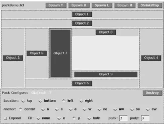
6.1.7 About the Pack Command . . . 241
6.1.8 An Introduction to the Grid Geometry Manager . . . . 243
6.1.9 Implementing a GUI as a Class . . . 245
6.1.10 A Simple Graphical Function Evaluator . . . 247
6.1.11 Exercises . . . 248
6.2 Adding GUIs to Scripts . . . 250
6.2.1 A Simulation and Visualization Script with a GUI . . 250
6.2.2 Improving the Layout . . . 253
6.2.3 Exercises . . . 256
6.3 A List of Common Widget Operations . . . 257
6.3.1 Frame . . . 259
6.3.2 Label . . . 260
6.3.3 Button . . . 262
6.3.4 Text Entry . . . 262
6.3.5 Balloon Help . . . 264
6.3.6 Option Menu . . . 265
6.3.7 Slider . . . 265
6.3.8 Check Button . . . 266
6.3.9 Making a Simple Megawidget . . . 266
6.3.10 Menu Bar . . . 267
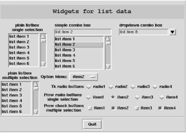
6.3.11 List Data . . . 269
6.3.12 Listbox . . . 269
6.3.13 Radio Button . . . 272
6.3.14 Combo Box . . . 274
6.3.15 Message Box . . . 275
6.3.16 User-Defined Dialogs . . . 277
6.3.17 Color-Picker Dialogs . . . 278
6.3.18 File Selection Dialogs . . . 279
6.3.19 Toplevel . . . 280
6.3.20 Some Other Types of Widgets . . . 281
6.3.21 Adapting Widgets to the User’s Resize Actions . . . 282
6.3.22 Customizing Fonts and Colors . . . 284
6.3.23 Widget Overview . . . 286
Table of Contents XV
7
Web Interfaces and CGI Programming
. . . . 2957.1 Introductory CGI Scripts . . . 296
7.1.1 Web Forms and CGI Scripts . . . 297
7.1.2 Generating Forms in CGI Scripts . . . 299
7.1.3 Debugging CGI Scripts . . . 301
7.1.4 A General Shell Script Wrapper for CGI Scripts . . . . 302
7.1.5 Security Issues . . . 304
7.2 Adding Web Interfaces to Scripts . . . 306
7.2.1 A Class for Form Parameters . . . 306
7.2.2 Calling Other Programs . . . 308
7.2.3 Running Simulations . . . 309
7.2.4 Getting a CGI Script to Work . . . 311
7.2.5 Using Web Applications from Scripts . . . 313
7.2.6 Exercises . . . 316
8
Advanced Python
. . . . 3198.1 Miscellaneous Topics . . . 319
8.1.1 Parsing Command-Line Arguments . . . 319
8.1.2 Platform-Dependent Operations . . . 322
8.1.3 Run-Time Generation of Code . . . 323
8.1.4 Exercises . . . 324
8.2 Regular Expressions and Text Processing . . . 326
8.2.1 Motivation . . . 326
8.2.2 Special Characters . . . 329
8.2.3 Regular Expressions for Real Numbers . . . 331
8.2.4 Using Groups to Extract Parts of a Text . . . 334
8.2.5 Extracting Interval Limits . . . 335
8.2.6 Extracting Multiple Matches . . . 339
8.2.7 Splitting Text . . . 344
8.2.8 Pattern-Matching Modifiers . . . 345
8.2.9 Substitution and Backreferences . . . 347
8.2.10 Example: Swapping Arguments in Function Calls . . . 348
8.2.11 A General Substitution Script . . . 351
8.2.12 Debugging Regular Expressions . . . 353
8.2.13 Exercises . . . 354
8.3 Tools for Handling Data in Files . . . 362
8.3.1 Writing and Reading Python Data Structures . . . 362
8.3.2 Pickling Objects . . . 364
8.3.3 Shelving Objects . . . 366
8.3.4 Writing and Reading Zip and Tar Archive Files . . . 366
8.3.5 Downloading Internet Files . . . 367
8.3.6 Binary Input/Output . . . 368
8.3.7 Exercises . . . 371
8.4 A Database for NumPy Arrays . . . 371
8.4.1 The Structure of the Database . . . 371
8.4.2 Pickling . . . 374
8.4.4 Shelving . . . 376
8.4.5 Comparing the Various Techniques . . . 377
8.5 Scripts Involving Local and Remote Hosts . . . 378
8.5.1 Secure Shell Commands . . . 378
8.5.2 Distributed Simulation and Visualization . . . 380
8.5.3 Client/Server Programming . . . 382
8.5.4 Threads . . . 382
8.6 Classes . . . 384
8.6.1 Class Programming . . . 384
8.6.2 Checking the Class Type . . . 388
8.6.3 Private Data . . . 389
8.6.4 Static Data . . . 390
8.6.5 Special Attributes . . . 390
8.6.6 Special Methods . . . 391
8.6.7 Multiple Inheritance . . . 392
8.6.8 Using a Class as a C-like Structure . . . 393
8.6.9 Attribute Access via String Names . . . 394
8.6.10 New-Style Classes . . . 394
8.6.11 Implementing Get/Set Functions via Properties . . . 395
8.6.12 Subclassing Built-in Types . . . 396
8.6.13 Building Class Interfaces at Run Time . . . 399
8.6.14 Building Flexible Class Interfaces . . . 403
8.6.15 Exercises . . . 409
8.7 Scope of Variables . . . 413
8.7.1 Global, Local, and Class Variables . . . 413
8.7.2 Nested Functions . . . 415
8.7.3 Dictionaries of Variables in Namespaces . . . 416
8.8 Exceptions . . . 418
8.8.1 Handling Exceptions . . . 419
8.8.2 Raising Exceptions . . . 420
8.9 Iterators . . . 421
8.9.1 Constructing an Iterator . . . 421
8.9.2 A Pointwise Grid Iterator . . . 423
8.9.3 A Vectorized Grid Iterator . . . 427
8.9.4 Generators . . . 428
8.9.5 Some Aspects of Generic Programming . . . 432
8.9.6 Exercises . . . 436
8.10 Investigating Efficiency . . . 437
8.10.1 CPU-Time Measurements . . . 437
8.10.2 Profiling Python Scripts . . . 441
8.10.3 Optimization of Python Code . . . 442
Table of Contents XVII
9
Fortran Programming with NumPy Arrays
. . . . 4519.1 Problem Definition . . . 451
9.2 Filling an Array in Fortran . . . 453
9.2.1 The Fortran Subroutine . . . 454
9.2.2 Building and Inspecting the Extension Module . . . 455
9.3 Array Storage Issues . . . 457
9.3.1 Generating an Erroneous Interface . . . 457
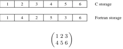
9.3.2 Array Storage in C and Fortran . . . 459
9.3.3 Input and Output Arrays as Function Arguments . . . 459
9.3.4 F2PY Interface Files . . . 466
9.3.5 Hiding Work Arrays . . . 470
9.4 Increasing Callback Efficiency . . . 470
9.4.1 Callbacks to Vectorized Python Functions . . . 471
9.4.2 Avoiding Callbacks to Python . . . 473
9.4.3 Compiled Inline Callback Functions . . . 474
9.5 Summary . . . 478
9.6 Exercises . . . 479
10 C and C++ Programming with NumPy Arrays
. . 48310.1 Automatic Interfacing of C/C++ Code . . . 484
10.1.1 Using F2PY . . . 485
10.1.2 Using Instant . . . 486
10.1.3 Using Weave . . . 487
10.2 C Programming with NumPy Arrays . . . 488
10.2.1 The Basics of the NumPy C API . . . 489
10.2.2 The Handwritten Extension Code . . . 491
10.2.3 Sending Arguments from Python to C . . . 492
10.2.4 Consistency Checks . . . 493
10.2.5 Computing Array Values . . . 494
10.2.6 Returning an Output Array . . . 496
10.2.7 Convenient Macros . . . 497
10.2.8 Module Initialization . . . 499
10.2.9 Extension Module Template . . . 500
10.2.10 Compiling, Linking, and Debugging the Module . . . 502
10.2.11 Writing a Wrapper for a C Function . . . 503
10.3 C++ Programming with NumPy Arrays . . . 506
10.3.1 Wrapping a NumPy Array in a C++ Object . . . 506
10.3.2 Using SCXX . . . 508
10.3.3 NumPy–C++ Class Conversion . . . 511
10.4 Comparison of the Implementations . . . 519
10.4.1 Efficiency . . . 519
10.4.2 Error Handling . . . 523
10.4.3 Summary . . . 524
11 More Advanced GUI Programming
. . . . 52911.1 Adding Plot Areas in GUIs . . . 529
11.1.1 The BLT Graph Widget . . . 530
11.1.2 Animation of Functions in BLT Graph Widgets . . . 536
11.1.3 Other Tools for Making GUIs with Plots . . . 538
11.1.4 Exercises . . . 539
11.2 Event Bindings . . . 541
11.2.1 Binding Events to Functions with Arguments . . . 542
11.2.2 A Text Widget with Tailored Keyboard Bindings . . . 544
11.2.3 A Fancy List Widget . . . 547
11.3 Animated Graphics with Canvas Widgets . . . 550
11.3.1 The First Canvas Encounter . . . 551
11.3.2 Coordinate Systems . . . 552
11.3.3 The Mathematical Model Class . . . 556
11.3.4 The Planet Class . . . 557
11.3.5 Drawing and Moving Planets . . . 559
11.3.6 Dragging Planets to New Positions . . . 560
11.3.7 Using Pmw’s Scrolled Canvas Widget . . . 564
11.4 Simulation and Visualization Scripts . . . 566
11.4.1 Restructuring the Script . . . 567
11.4.2 Representing a Parameter by a Class . . . 569
11.4.3 Improved Command-Line Script . . . 583
11.4.4 Improved GUI Script . . . 584
11.4.5 Improved CGI Script . . . 585
11.4.6 Parameters with Physical Dimensions . . . 586
11.4.7 Adding a Curve Plot Area . . . 588
11.4.8 Automatic Generation of Scripts . . . 589
11.4.9 Applications of the Tools . . . 590
11.4.10 Allowing Physical Units in Input Files . . . 596
11.4.11 Converting Input Files to GUIs . . . 601
12 Tools and Examples
. . . .60512.1 Running Series of Computer Experiments . . . 605
12.1.1 Multiple Values of Input Parameters . . . 606
12.1.2 Implementation Details . . . 609
12.1.3 Further Applications . . . 614
12.2 Tools for Representing Functions . . . 618
12.2.1 Functions Defined by String Formulas . . . 618
12.2.2 A Unified Interface to Functions . . . 623
12.2.3 Interactive Drawing of Functions . . . 629
12.2.4 A Notebook for Selecting Functions . . . 633
12.3 Solving Partial Differential Equations . . . 640
12.3.1 Numerical Methods for 1D Wave Equations . . . 641
12.3.2 Implementations of 1D Wave Equations . . . 644
12.3.3 Classes for Solving 1D Wave Equations . . . 651
12.3.4 A Problem Solving Environment . . . 657
Table of Contents XIX
12.3.6 Implementations of 2D Wave Equations . . . 666
12.3.7 Exercises . . . 675
A Setting up the Required Software Environment
. . . 677A.1 Installation on Unix Systems . . . 677
A.1.1 A Suggested Directory Structure . . . 677
A.1.2 Setting Some Environment Variables . . . 678
A.1.3 Installing Tcl/Tk and Additional Modules . . . 679
A.1.4 Installing Python . . . 680
A.1.5 Installing Python Modules . . . 681
A.1.6 Installing Gnuplot . . . 683
A.1.7 Installing SWIG . . . 684
A.1.8 Summary of Environment Variables . . . 684
A.1.9 Testing the Installation of Scripting Utilities . . . 685
A.2 Installation on Windows Systems . . . 685
B Elements of Software Engineering
. . . . 689B.1 Building and Using Modules . . . 689
B.1.1 Single-File Modules . . . 689
B.1.2 Multi-File Modules . . . 693
B.1.3 Debugging and Troubleshooting . . . 694
B.2 Tools for Documenting Python Software . . . 696
B.2.1 Doc Strings . . . 696
B.2.2 Tools for Automatic Documentation . . . 698
B.3 Coding Standards . . . 702
B.3.1 Style Guide . . . 702
B.3.2 Pythonic Programming . . . 706
B.4 Verification of Scripts . . . 711
B.4.1 Automating Regression Tests . . . 711
B.4.2 Implementing a Tool for Regression Tests . . . 715
B.4.3 Writing a Test Script . . . 719
B.4.4 Verifying Output from Numerical Computations . . . . 720
B.4.5 Automatic Doc String Testing . . . 724
B.4.6 Unit Testing . . . 726
B.5 Version Control Management . . . 728
B.5.1 Mercurial . . . 729
B.5.2 Subversion . . . 732
B.6 Exercises . . . 734
Bibliography
. . . . 739Exercise 2.1 Become familiar with the electronic documentation . . . 31
Exercise 2.2 Extend Exercise 2.1 with a loop . . . 43
Exercise 2.3 Find five errors in a script . . . 43
Exercise 2.4 Basic use of control structures . . . 43
Exercise 2.5 Use standard input/output instead of files . . . 44
Exercise 2.6 Read streams of (x, y) pairs from the command line . . . . 45
Exercise 2.7 Test for specific exceptions . . . 45
Exercise 2.8 Sum columns in a file . . . 45
Exercise 2.9 Estimate the chance of an event in a dice game . . . 45
Exercise 2.10 Determine if you win or loose a hazard game . . . 46
Exercise 2.11 Generate an HTML report from thesimviz1.py script . . 55
Exercise 2.12 Generate a LATEX report from thesimviz1.py script . . . . 56
Exercise 2.13 Compute time step values in thesimviz1.py script . . . 57
Exercise 2.14 Use Matlab for curve plotting in thesimviz1.py script . . 57
Exercise 2.15 Combine curves from two simulations in one plot . . . 61
Exercise 2.16 Combine two-column data files to a multi-column file . . . 71
Exercise 2.17 Read/write Excel data files in Python . . . 72
Exercise 3.1 Write format specifications in printf-style . . . 106
Exercise 3.2 Write your own function for joining strings . . . 106
Exercise 3.3 Write an improved function for joining strings . . . 106
Exercise 3.4 Never modify a list you are iterating on . . . 107
Exercise 3.5 Make a specialized sort function . . . 107
Exercise 3.6 Check if your system has a specific program . . . 108
Exercise 3.7 Find the paths to a collection of programs . . . 108
Exercise 3.8 Use Exercise 3.7 to improve thesimviz1.pyscript . . . 109
Exercise 3.9 Use Exercise 3.7 to improve theloop4simviz2.py script . 109 Exercise 3.10 Find the version number of a utility . . . 109
Exercise 3.11 Automate execution of a family of similar commands . . . 125
Exercise 3.12 Remove temporary files in a directory tree . . . 125
Exercise 3.13 Find old and large files in a directory tree . . . 126
Exercise 3.14 Remove redundant files in a directory tree . . . 126
Exercise 3.15 Annotate a filename with the current date . . . 127
Exercise 3.16 Automatic backup of recently modified files . . . 127
Exercise 3.17 Search for a text in files with certain extensions . . . 128
Exercise 3.18 Search directories for plots and make HTML report . . . . 128
Exercise 3.19 Fix Unix/Windows Line Ends . . . 129
Exercise 4.1 Matrix-vector multiply with NumPy arrays . . . 146
Exercise 4.2 Work with slicing and matrix multiplication . . . 146
Exercise 4.3 Assignment and in-place NumPy array modifications . . . 147
XXII List of Exercises
Exercise 4.5 Vectorize a numerical integration rule . . . 150
Exercise 4.6 Vectorize a formula containing an if condition . . . 151
Exercise 4.7 Slicing of two-dimensional arrays . . . 151
Exercise 4.8 Implement Exercise 2.9 using NumPy arrays . . . 168
Exercise 4.9 Implement Exercise 2.10 using NumPy arrays . . . 169
Exercise 4.10 Replace lists by NumPy arrays inconvert2.py . . . 169
Exercise 4.11 Use Easyviz in thesimviz1.py script . . . 169
Exercise 4.12 Extension of Exercise 2.8 . . . 169
Exercise 4.13 NumPy arrays and binary files . . . 169
Exercise 4.14 One-dimensional Monte Carlo integration . . . 169
Exercise 4.15 Higher-dimensional Monte Carlo integration . . . 170
Exercise 4.16 Load data file into NumPy array and visualize . . . 171
Exercise 4.17 Analyze trends in the data from Exercise 4.16 . . . 171
Exercise 4.18 Evaluate a function over a 3D grid . . . 171
Exercise 4.19 Evaluate a function over a plane or line in a 3D grid . . . . 172
Exercise 5.1 Implement a numerical integration rule in F77 . . . 214
Exercise 5.2 Implement a numerical integration rule in C . . . 214
Exercise 5.3 Implement a numerical integration rule in C++ . . . 214
Exercise 6.1 Modify the Scientific Hello World GUI . . . 248
Exercise 6.2 Change the layout of the GUI in Exercise 6.1 . . . 248
Exercise 6.3 Control a layout with the grid geometry manager . . . 249
Exercise 6.4 Make a demo of Newton’s method . . . 250
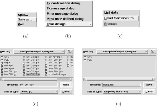
Exercise 6.5 Program withPmw.EntryField inhwGUI10.py . . . 256
Exercise 6.6 Program withPmw.EntryField insimvizGUI2.py . . . 256
Exercise 6.7 Replace Tkinter variables by set/get-like functions . . . 256
Exercise 6.8 Usesimviz1.pyas a module insimvizGUI2.py. . . 256
Exercise 6.9 Apply Matlab for visualization insimvizGUI2.py . . . 257
Exercise 6.10 Program withPmw.OptionMenu insimvizGUI2.py . . . 289
Exercise 6.11 Study the nonlinear motion of a pendulum . . . 289
Exercise 6.12 Add error handling with an associated message box . . . . 290
Exercise 6.13 Add a message bar to a balloon help . . . 290
Exercise 6.14 Select a file from a list and perform an action . . . 291
Exercise 6.15 Make a GUI for finding and selecting font names . . . 291
Exercise 6.16 Launch a GUI when command-line options are missing . 292 Exercise 6.17 Write a GUI for Exercise 3.14 . . . 292
Exercise 6.18 Write a GUI for selecting files to be plotted . . . 293
Exercise 6.19 Write an easy-to-use GUI generator . . . 293
Exercise 7.1 Write a CGI debugging tool . . . 316
Exercise 7.2 Make a web calculator . . . 316
Exercise 7.3 Make a web application for registering participants . . . 317
Exercise 7.4 Make a web application for numerical experiments . . . 317
Exercise 7.5 Become a “nobody” user on a web server . . . 317
Exercise 8.1 Use the getopt/optparse module insimviz1.py . . . 324
Exercise 8.2 Store command-line options in a dictionary . . . 325
Exercise 8.4 A grep script . . . 354
Exercise 8.5 Experiment with a regex for real numbers . . . 355
Exercise 8.6 Find errors in regular expressions . . . 355
Exercise 8.7 Generate data from a user-supplied formula . . . 356
Exercise 8.8 Explain the behavior of regular expressions . . . 356
Exercise 8.9 Edit extensions in filenames . . . 357
Exercise 8.10 Extract info from a program code . . . 357
Exercise 8.11 Regex for splitting a pathname . . . 357
Exercise 8.12 Rename a collection of files according to a pattern . . . 358
Exercise 8.13 Reimplement there.findall function . . . 358
Exercise 8.14 Interpret a regex code and find programming errors . . . . 358
Exercise 8.15 Automatic fine tuning of PostScript figures . . . 359
Exercise 8.16 Transform a list of lines to a list of paragraphs . . . 360
Exercise 8.17 Copy computer codes into documents . . . 360
Exercise 8.18 A very useful script for all writers . . . 361
Exercise 8.19 Read Fortran 90 files with namelists . . . 361
Exercise 8.20 Automatic update of function calls in C++ files . . . 361
Exercise 8.21 Read/write (x, y) pairs from/to binary files . . . 371
Exercise 8.22 Use the XDR format in the script from Exercise 8.21 . . . 371
Exercise 8.23 Archive all files needed in a LATEX document . . . 371
Exercise 8.24 Using a web site for distributed simulation . . . 381
Exercise 8.25 Convert data structures to/from strings . . . 409
Exercise 8.26 Implement a class for vectors in 3D . . . 410
Exercise 8.27 Extend the class from Exericse 8.26 . . . 410
Exercise 8.28 Make a tuple with cyclic indices . . . 411
Exercise 8.29 Make a dictionary type with ordered keys . . . 411
Exercise 8.30 Make a smarter integration function . . . 412
Exercise 8.31 Equip classGrid2Dwith subscripting . . . 412
Exercise 8.32 Extend the functionality of classGrid2D. . . 412
Exercise 8.33 Make a boundary iterator in a 2D grid . . . 436
Exercise 8.34 Make a generator for odd numbers . . . 436
Exercise 8.35 Make a class for sparse vectors . . . 436
Exercise 9.1 Extend Exercise 5.1 with a callback to Python . . . 479
Exercise 9.2 Compile callback functions in Exercise 9.1 . . . 479
Exercise 9.3 Smoothing of time series . . . 480
Exercise 9.4 Smoothing of 3D data . . . 480
Exercise 9.5 Type incompatibility between Python and Fortran . . . 481
Exercise 9.6 Problematic callbacks to Python from Fortran . . . 481
Exercise 9.7 Array look-up efficiency: Python vs. Fortran . . . 482
Exercise 10.1 Extend Exercise 5.2 or 5.3 with a callback to Python . . . 525
Exercise 10.2 Investigate the efficiency of vector operations . . . 525
Exercise 10.3 Debug a C extension module . . . 525
Exercise 10.4 Make callbacks to vectorized Python functions . . . 526
Exercise 10.5 Avoid Python callbacks in extension modules . . . 526
XXIV List of Exercises
Exercise 10.7 Apply SWIG to an array class in C++ . . . 526
Exercise 10.8 Build a dictionary in C . . . 526
Exercise 10.9 Make a C module for computing random numbers . . . 527
Exercise 10.10 Almost automatic generation of C extension modules . . . 527
Exercise 10.11 Introduce C++ array objects in Exercise 10.10 . . . 528
Exercise 10.12 Introduce SCXX in Exercise 10.11 . . . 528
Exercise 11.1 Incorporate a BLT graph widget insimviz1.py. . . 539
Exercise 11.2 Plot a two-column datafile in a Pmw.Blt widget . . . 539
Exercise 11.3 Use a BLT graph widget insimvizGUI2.py. . . 539
Exercise 11.4 Extend Exercise 11.3 to handle multiple curves . . . 539
Exercise 11.5 Use a BLT graph widget in Exercise 6.4 . . . 539
Exercise 11.6 Interactive dump of snapshot plots in an animation . . . . 540
Exercise 11.7 Extend theanimate.py GUI . . . 540
Exercise 11.8 Animate a curve in a BLT graph widget . . . 541
Exercise 11.9 Add animations to the GUI in Exercise 11.5 . . . 541
Exercise 11.10 Extend the GUI in Exercise 6.17 with a fancy list . . . 550
Exercise 11.11 Remove canvas items . . . 566
Exercise 11.12 Introduce properties in classParameters. . . 580
Exercise 11.13 Convert command file into Python objects . . . 600
Exercise 12.1 Allow multiple values of parameters in input files . . . 617
Exercise 12.2 Turn mathematical formulas into Fortran functions . . . 628
Exercise 12.3 Move a wave source during simulation . . . 675
Exercise 12.4 Include damping in a 1D wave simulator . . . 675
Exercise 12.5 Add a NumPy database to a PDE simulator . . . 675
Exercise 12.6 Use iterators in finite difference schemes . . . 675
Exercise 12.7 Set vectorized boundary conditions in 3D grids . . . 675
Exercise B.1 Make a Python module of simviz1.py . . . 734
Exercise B.2 Pack modules and packages using Distutils . . . 735
Exercise B.3 Distribute mixed-language code using Distutils . . . 735
Exercise B.4 Use tools to document the script in Exercise 3.14 . . . 735
Exercise B.5 Make a regression test for a trivial script . . . 735
Exercise B.6 Repeat Exercise B.5 using the test script tools . . . 735
Exercise B.7 Make a regression test for a script with I/O . . . 735
Exercise B.8 Make a regression test for the script in Exercise 3.14 . . . 736
Exercise B.9 Approximate floats in Exercise B.5 . . . 736
Exercise B.10 Make tests for grid iterators . . . 736
Exercise B.11 Make a tar/zip archive of files associated with a script . . 736
Introduction
In this introductory chapter we first look at some arguments why scripting is a promising programming style for computational scientists and engineers and how scripting differs from more traditional programming in Fortran, C, C++, C#, and Java. The chapter continues with a section on how to set up your software environment such that you are ready to get started with the introduction to Python scripting in Chapter 2. Eager readers who want to get started with Python scripting as quickly as possible can safely jump to Chapter 1.2 to set up their environment and get ready to dive into examples in Chapter 2.
1.1
Scripting versus Traditional Programming
The purpose of this section is to point out differences between scripting and traditional programming. These are two quite different programming styles, often with different goals and utilizing different types of programming lan-guages. Traditional programming, also often referred to assystem program-ming, refers to building (usually large, monolithic) applications (systems) using languages such as Fortran1, C, C++, C#, or Java. In the context of this book, scripting means programming at a high and flexible abstraction level, utilizing languages like Perl, Python, Ruby, Scheme, or Tcl. Very of-ten the script integrates operation system actions, text processing and report writing, with functionality in monolithic systems. There is a continuous tran-sition from scripting to traditional programming, but this section will be more focused on the features that distinguish these programming styles.
Hopefully, the present section motivates the reader to get started with scripting in Chapter 2. Much of what is written in this section may make more sense after you have experience with scripting, so you are encouraged to go back and read it again at a later stage to get a more thorough view of how scripting fits in with other programming techniques.
1 By “Fortran” I mean all versions of Fortran (77, 90/95, 2003), unless a specific
2 1. Introduction
1.1.1
Why Scripting is Useful in Computational Science
Scientists Are on the Move. During the last decade, the popularity of sci-entific computing environments such as IDL, Maple, Mathematica, Matlab, Octave, and S-PLUS/R has increased considerably. Scientists and engineers simply feel more productive in such environments. One reason is the simple and clean syntax of the command languages in these environments. Another factor is the tight integration of simulation and visualization: in Maple, Mat-lab, S-PLUS/R and similar environments you can quickly and conveniently visualize what you just have computed.
Build Your Own Environment. One problem with the mentioned environ-ments is that they do not work, at least not in an easy way, with other types of numerical software and visualization systems. Many of the environment-specific programming languages are also quite simple or primitive. At this point scripting in Python comes in. Python offers the clean and simple syn-tax of the popular scientific computing environments, the language is very powerful, and there are lots of tools for gluing your favorite simulation, vi-sualization, and data analysis programs the way you want. Phrased differ-ently, Python allows you to build your own Matlab-like scientific computing environment, tailored to your specific needs and based on your favorite high-performance Fortran, C, or C++ codes.
Scientific Computing Is More Than Number Crunching. Many computa-tional scientists work with their own numerical software development and realize that much of the work is not only writing computationally intensive number-crunching loops. Very often programming is about shuffling data in and out of different tools, converting one data format to another, extracting numerical data from a text, and administering numerical experiments involv-ing a large number of data files and directories. Such tasks are much faster to accomplish in a language like Python than in Fortran, C, C++, C#, or Java. Chapter 3 presents lots of examples in this context.
Graphical User Interfaces. GUIs are becoming increasingly more important in scientific software, but (normally) computational scientists and engineers have neither the interest nor the time to read thick books about GUI pro-gramming. What you need is a quick “how-to” description of wrapping GUIs to your applications. The Tk-based GUI tools available through Python make it easy to wrap existing programs with a GUI. Chapter 6 provides an intro-duction.
Some relevant demo examples can be found in Chapters 2.3, 6.2, 7.2, 11.4, and 12.3.
Modern Interfaces to Old Simulation Codes. Many Fortran and C program-mers want to take advantage of new programming paradigms and languages, but at the same time they want to reuse their old well-tested and efficient codes. Instead of migrating these codes to C++, recent Fortran versions, or Java, one can wrap the codes with a scripting interface. Calling Fortran, C, or C++ from Python is particularly easy, and the Python interfaces can take advantage of object-oriented design and simple coupling to GUIs, visualiza-tion, or other programs. Computing with your Fortran or C libraries from these interfaces can then be done either in short scripts or in a fully interac-tive manner through a Python shell. Roughly speaking, you can use Python interfaces to your existing libraries as a way of creating your own tailored problem solving environment. Chapter 5 explains how Python code can call Fortran, C, and C++.
Unix Power on Windows. We also mention that many computational sci-entists are tied to and take great advantage of the Unix operating system. Moving to Microsoft Windows environments can for many be a frustrating process. Scripting languages are very much inspired by Unix, yet cross plat-form. Using scripts to create your working environment actually gives you the power of Unix (and more!) also on Windows and Macintosh machines. In fact, a script-based working environment can give you the combined power of the Unix and Windows/Macintosh working styles. Many examples of operating system interaction through Python are given in Chapter 3.
Python versus Matlab. Some readers may wonder why an environment such as Matlab or something similar (like Octave, Scilab, Rlab, Euler, Tela, Yorick) is not sufficient. Matlab is a de facto standard, which to some extent offers many of the important features mentioned in the previous paragraphs. Matlab and Python have indeed many things in common, including no declaration of variables, simple and convenient syntax, easy creation of GUIs, and gluing of simulation and visualization. Nevertheless, in my opinion Python has some clear advantageous over Matlab and similar environments:
– the Python programming language is more powerful,
– the Python environment is completely open and made for integration with external tools,
– a complete toolbox/module with lots of functions and classes can be contained in a single file (in contrast to a bunch of M-files),
– transferring functions as arguments to functions is simpler,
– nested, heterogeneous data structures are simple to construct and use, – object-oriented programming is more convenient,
4 1. Introduction
– scalar functions work with array arguments to a larger extent (without modifications of arithmetic operators),
– the source is free and runs on more platforms.
Having said this, we must add that Matlab appears as a more self-contained environment, while Python needs to combined with several additional pack-ages to form an environment of competitive functionality. There is an inter-face pymat that allows Python programs to use Matlab as a computational and graphics engine (see Chapter 4.4.3). At the time of this writing, Python’s support for numerical computing and visualization is rapidly growing, espe-cially through the SciPy project (see Chapter 4.4.2).
1.1.2
Classification of Programming Languages
It is convenient to have a term for the languages used for traditional scientific programming and the languages used for scripting. We propose to use type-safe languages and dynamically typed languages, respectively. These terms distinguish the languages by the flexibility of the variables, i.e., whether vari-ables must be declared with a specific type or whether varivari-ables can hold data of any type. This is a clear and important distinction of the functionality of the two classes of programming languages.
Many other characteristics are candidates for classifying these languages. Some speak about compiled languages versus interpreted languages (Java complicates these matters, as it is type-safe, but have the nature of being both interpreted and compiled). Scripting languages and system program-ming languages are also very common terms [27], i.e., classifying languages by their typical associated programming style. Others refer to high-level and low-level languages. High and low in this context implies no judgment of quality. High-level languages are characterized by constructs and data types close to natural language specifications of algorithms, whereas low-level lan-guages work with constructs and data types reflecting the hardware level. This distinction may well describe the difference between Perl and Python, as high-level languages, versus C and Fortran, as low-level languages. C++, C#, and Java come somewhat in between. High-level languages are also often referred to as very high-level languages, indicating the problem of choosing a common scale when measuring the level of languages.
1.1.3
Productive Pairs of Programming Languages
Unix and C. Unix evolved to be a very productive software development environment based on two programming tools of different nature: the classical system programming language C for CPU-critical tasks, often involving non-trivial data structures, and the Unix shell for gluing C programs to form new applications. With only a handful of basic C programs as building blocks, a user can solve a new problem by writing a tailored shell program combining existing tools in a simple way. For example, there is no basic Unix tool that enables browsing a sorted list of the disk usage in the directories of a user, but it is trivial to combine three C programs,dufor summarizing disk usage, sortfor sorting lines of text, and lessfor browsing text files, together with the pipe functionality of Unix shells, to build the desired tool as a one-line shell instruction:
du -a $HOME | sort -rn | less
In this way, we glue three programs that are in principle completely indepen-dent of each other. This is the power of Unix in a nutshell. Without the gluing capabilities of Unix shells, we would need to write a tailored C program, of a much larger complexity, to solve the present problem.
A Unix command interpreter, or shell as it is normally called, provides a language for gluing applications. There are many shells: Bourne shell (sh) and C shell (csh) are classical, whereas Bourne Again shell (bash), Korn shell (ksh), and Z shell (zsh) are popular modern shells. A program written in a shell is often referred to as a script. Although the Unix shells have many useful high-level features that contribute to keep the size of scripts small, the shells are quite primitive programming languages, at least when viewed by modern programmers.
C is a low-level language, often claimed to be designed for computers and not humans. However, low-level system programming languages like C and Fortran 77 were introduced as alternatives to the much more low-level as-sembly languages and have been successful for making computationally fast code, yet with a reasonable abstraction level. Fortran 77 and C give nearly complete control of memory usage and CPU-critical program segments, but the amount of details at a low code level is unfortunately huge. The need for programming tools that increase the human productivity led to a devel-opment of more powerful languages, both for classical system programming and for scripting.
6 1. Introduction
object-oriented and generic programming. VisualBasic is also a richer lan-guage than Unix shells.
Java. Especially for tasks related to Internet programming, Java was from the mid 1990s taking over as the preferred language for building large software systems. Many regard JavaScript as some kind of scripting companion in web pages. PHP and Java are also a popular pair. However, Java is much of a self-contained language, and being simpler and safer to apply than C++, it has become very popular and widespread for classical system programming. A promising scripting companion to Java is Jython, the Java implementation of Python. On the .NET platform, C# plays a Java-like role and can be combined with Python to form a pair of system and scripting language.
Modern Scripting Languanges. During the last decade several powerful dy-namically typed languages have emerged and developed to a mature state. Bash, Perl, Python (and Jython), Ruby, Scheme, and Tcl are examples of general-purpose, modern, widespread languages that are popular for script-ing tasks. PHP is a related language, but more specialized towards makscript-ing web applications.
1.1.4
Gluing Existing Applications
Dynamically typed languages are often used for gluing stand-alone applica-tions (typically coded in a type-safe language) and offer for this purpose rich interfaces to operating system functionality, file handling, and text process-ing. A relevant example for computational scientists and engineers is gluing a simulation program, a visualization program, and perhaps a data analysis program, to form an easy-to-use tool for problem solving. Running a program, grabbing and modifying its output, and directing data to another program are central tasks when gluing applications, and these tasks are easier to ac-complish in a language like Python than in Fortran, C, C++, C#, or Java. A script that glues existing components to form a new application often needs a graphical user interface (GUI), and adding a GUI is normally a simpler task in dynamically typed languages than in the type-safe languages.
at-tractive for high-performance computing. The topic is treated in Chapters 9 and 10.
1.1.5
Scripting Yields Shorter Code
Powerful dynamically typed languages, such as Python, support numerous high-level constructs and data structures enabling you to write programs that are significantly shorter than programs with corresponding functionality coded in Fortran, C, C++, C#, or Java. In other words, more work is done (on average) per statement. A simple example is reading ana prioriunknown number of real numbers from a file, where several numbers may appear at one line and blank lines are permitted. This task is accomplished by two Python statements2:
F = open(filename, ’r’); n = F.read().split()
Trying to do this in Fortran, C, C++, or Java requires at least a loop, and in some of the languages several statements needed for dealing with a variable number of reals per line.
As another example, think about reading a complex number expressed in a text format like(-3.1,4). We can easily extract the real part−3.1 and the imaginary part 4 from the string (-3.1,4) using a regular expression, also when optional whitespace is included in the text format. Regular expressions are particularly well supported by dynamically typed languages. The relevant Python statements read3
m = re.search(r’\(\s*([^,]+)\s*,\s*([^,]+)\s*\)’, ’ (-3.1, 4) ’) re, im = [float(x) for x in m.groups()]
We can alternatively strip off the parenthesis and then split the string’-3.1,4’ with respect to the comma character:
m = ’ (-3.1, 4) ’.strip()[1:-1]
re, im = [float(x) for x in m.split(’,’)]
This solution applies string operations and a convenient indexing syntax in-stead of regular expressions. Extracting the real and imaginary numbers in Fortran or C code requires many more instructions, doing string searching and manipulations at the character array level.
The special text of comma-separated numbers enclosed in parenthesis, like (-3.1,4), is a valid textual representation of a standard list (tuple) in
2 Do not try to understand the details of the statements. The size of the code is
what matters at this point. The meaning of the statements will be evident from Chapter 2.
3 The code examples may look cryptic for a novice, but the meaning of the sequence
8 1. Introduction
Python. This allows us in fact to convert the text to a list variable and from there extract the list elements by a very simple code:
re, im = eval(’(-3.1, 4)’)
The ability to convert textual representation of lists (including nested, het-erogeneous lists) to list variables is a very convenient feature of scripting. In Python you can have a variableqholding, e.g., a list of various data and say s=str(q) to convertqto a stringsand q=eval(s)to convert the string back to a list variable again. This feature makes writing and reading non-trivial data structures trivial, which we demonstrate in Chapter 8.3.1.
Ousterhout’s article [27] about scripting refers to several examples where the code-size ratio and the implementation-time ratio between type-safe lan-guages and the dynamically typed Tcl language vary from 2 to 60, in favor of Tcl. For example, the implementation of a database application in C++ took two months, while the reimplementation in Tcl, with additional functional-ity, took only one day. A database library was implemented in C++ during a period of 2-3 months and reimplemented in Tcl in about one week. The Tcl implementation of an application for displaying oil well curves required two weeks of labor, while the reimplementation in C needed three months. Another application, involving a simulator with a graphical user interface, was first implemented in Tcl, requiring 1600 lines of code and one week of labor. A corresponding Java version, with less functionality, required 3400 lines of code and 3-4 weeks of programming.
1.1.6
Efficiency
Scripts are first compiled to hardware-independent byte-code and then the byte-code isinterpreted. Type-safe languages, with the exception of Java, are compiled in the sense that all code is nailed down to hardware-dependent machine instructions before the program is executed. The interpreted, high-level, flexible data structures used in scripts imply a speed penalty, especially when traversing data structures of some size [6].
is that in the area of text processing, dynamically typed languages will often provide optimal efficiency both from a human and a computer point of view. Another attractive feature of dynamically typed languages is that they were designed for migrating CPU-critical code segments to C, C++, or For-tran. This can often resolve bottlenecks, especially in numerical computing. If you can solve your problem using, for example, fixed-size, contiguous arrays and traverse these arrays in a C, C++, or Fortran code, and thereby uti-lize the compilers’ sophisticated optimization techniques, the compiled code will run much faster than the similar script code. The speed-up we are talk-ing about here can easily be a factor of 100 (Chapters 9 and 10 presents examples).
1.1.7
Type-Specification (Declaration) of Variables
Type-safe languages require each variable to be explicitly declared with a specific type. The compiler makes use of this information to control that the right type of data is combined with the right type of algorithms. Some refer to statically typed and strongly typed languages. Static, being opposite of dynamic, means that a variable’s type is fixed at compiled time. This distinguishes, e.g., C from Python. Strong versus weak typing refers to if something of one type can be automatically used as another type, i.e., if implicit type conversion can take place. Variables in Perl may be weakly typed in the sense that
$b = ’1.2’; $c = 5.1*$b
is valid:$b gets converted from a string to a float in the multiplication. The same operation in Python is not legal, a string cannot suddenly act as a float4.
The advantage of type-safe languages is less bugs and safer programming, at a cost of decreased flexibility. In large projects with many programmers the static typing certainly helps managing complexity. Nevertheless, reuse of code is not always well supported by static typing since a piece of code only works with a particular type of data. Object-oriented and especially generic programming provide important tools to relax the rigidity of a statically typed environment.
In dynamically typed languages variables are not declared to be of any type, and there are noa priorirestrictions on how variables and functions are combined. When you need a variable, simply assign it a value – there is no need to mention the type. This gives great flexibility, but also undesired side effects from typing errors. Fortunately, dynamically typed languages usually perform extensive run-time checks (at a cost of decreased efficiency, of course)
4 With user-defined types in Python you are free to control implicit type conversion
10 1. Introduction
for consistent use of variables and functions. At least experienced program-mers will not be annoyed by errors arising from the lack of static typing: they will easily recognize typos or type mismatches from the run-time messages. The benefits of no explicit typing is that a piece of code can be applied in many contexts. This reduces the amount of code and thereby the number of bugs.
Here is an example of a generic Python function for dumping a data structure with a leading text:
def debug(leading_text, variable):
if os.environ.get(’MYDEBUG’, ’0’) == ’1’: print leading_text, variable
The function performs the print action only if the environment variable MYDEBUG is defined and has the value ’1’. By adjusting MYDEBUG in the op-erating system environment one can turn on and off the output fromdebug in any script.
The main point here is that the debug function actually works with any built-in data structure. We may send integers, floating-point numbers, com-plex numbers, arrays, and nested heterogeneous lists of user-defined objects (provided these have defined how to print themselves). With three lines of code we have made a very convenient tool. Such quick and useful code devel-opment is typical for scripting.
In a sense, templates in C++ mimics the nature of dynamically typed languages. The similar function in C++ reads
template <class T>
void debug(std::ostream& o,
const std::string& leading_text, const T& variable)
{
char* c = getenv("MYDEBUG"); bool defined = false;
if (c != NULL) { // if MYDEBUG is defined ...
if (std::string(c) == "1") { // if MYDEBUG is true ... defined = true;
} }
if (defined) {
o << leading_text << " " << variable << std::endl; }
}
In Fortran, C, and Java one needs to make different versions of debug for different types of the variablevariable.
which implies some work. The advantage is that we (and the compiler) have full control of what types that are allowed to be sent to debug. The Python debug function is much quicker to write and use, but we have no control of the type of variables that we try to print. For the present example this is irrelevant, but in large systems unintended transactions of objects may be critical. Static typing may then help, at the cost quite some extra work.
1.1.8
Flexible Function Interfaces
Problem solving environments such as IDL, Maple, Mathematica, Matlab, Octave, Scilab, and S-PLUS/R have simple-to-use command languages. One particular feature of these command languages, which enhances user friend-liness, is the possibility of using keyword or named arguments in function calls. As an illustration, consider a typical plot session5
f = calculate(...) # calculate something plot(f)
Whatever we calculate is stored inf, andplotacceptsfvariables of different types. In the simple plot(f) call, the function relies on default options for axis, labels, etc. More control is obtained by adding parameters in theplot call, e.g.,
plot(f, label=’elevation’, xrange=[0,10])
Here we specify a label to mark the curve and the extent of the x axis. Arguments with a name, saylabel, and a value, say’elevation’, are called keyword or named arguments. The advantage of such arguments is three-fold: (i) the user can specify just a few arguments and rely on default values for the rest, (ii) the sequence of the arguments is arbitrary, and (iii) the keywords help to document and explain the call. The more experienced user will often need to fine tune a plot, and in that case a range of additional arguments can be specified, for instance something like
plot(f, label=’elevation’, xrange=[0,10], title=’Variable bottom’, linetype=’dashed’, linecolor=’red’, yrange=[-1,1])
Python offers keyword arguments in functions, exactly as explained here. The plotcalls are in fact written with Python syntax (but theplotfunction itself is not a built-in Python feature: it is here supposed to be some user-defined function).
An argument can be of different types inside the plot function. Con-sider, for example, the xrange parameter. One could offer the specification of this parameter in several ways: (i) as a list [xmin,xmax], (ii) as a string
5 In this book, three dots (...) are used to indicate some irrelevant code that is
12 1. Introduction
’xmin:xmax’, or (iii) as a single floating-point number xmax, assuming that the minimum value is zero. These three cases can easily be dealt with inside theplot function, because Python enables checking the type ofxrange (the details are explained in Chapter 3.2.11).
Some functions,debugin Chapter 1.1.7 being an example, accept any type of argument, but Python issues run-time error messages when an operation is incompatible with the supplied type of argument. Theplotfunction above accepts only a limited set of argument types and could convert different types to a uniform representation (floating-point numbers xmin and xmax) within the function.
The nature and functionality of Python give you a full-fledged, advanced programming language at disposal, with the clean and easy-to-use interface syntax that has obtained great popularity through environments like Maple and Matlab. The function programming interface offered by type-safe lan-guages is more comprehensive, less flexible, and less user friendly. Having said this, we should add that user friendliness has, of course, many aspects and depends on personal taste. Static typing and comprehensive syntax may provide a reliability that some people find more user friendly than the pro-gramming style we advocate in this text.
1.1.9
Interactive Computing
Many of the most popular computational environments, such as IDL, Maple, Matlab, and S-PLUS/R, offer interactive computing. The user can type a command and immediately see the effect of it. Previous commands can quickly be recalled and edited on the fly. Since mistakes are easily discovered and cor-rected, interactive environments are ideal for exploring the steps of a compu-tational problem. When all details of the computations are clear, the com-mands can be collected in a file and run as a program.
Python offers an interactive shell, which provides the type of interactive environment just described. A very simple session could do some basic cal-culations:
>>> from math import * >>> w=1
>>> sin(w*2.5)*cos(1+w*3) -0.39118749925811952
The first line gives us access to functions like sin and cos. The next line defines a variablew, which is used in the computations in the proceeding line. User input follows after the >>> prompt, while the result of a command is printed without any prompt.
A less trival session could involve integrals of the Bessel functions Jn(x): >>> from scipy.special i