DOI:10.1051/0004-6361/201730757 c
ESO 2017
Astronomy
&
Astrophysics
Are over-massive haloes of ultra-diffuse galaxies consistent
with extended MOND?
Alistair O. Hodson and Hongsheng Zhao
School of Physics and Astronomy, University of St Andrews, St Andrews KY16 9SS, UK e-mail:[email protected]
Received 9 March 2017/Accepted 24 August 2017
ABSTRACT
Aims.A sample of Coma cluster ultra-diffuse galaxies (UDGs) are modelled in the context of extended modified Newtonian dynamics (EMOND) with the aim to explain the large dark matter-like effect observed in these cluster galaxies.
Methods.We first built a model of the Coma cluster in the context of EMOND using gas and galaxy mass profiles from the literature. Assuming that the dynamical mass of the UDGs satisfies the fundamental manifold of other ellipticals and that the UDG stellar mass-to-light ratio matches their colour, we then verified the EMOND formulation by comparing two predictions of the baryonic mass of UDGs.
Results.We find that EMOND can explain the UDG mass, within the expected modelling errors, if they lie on the fundamental manifold of ellipsoids, but given that measurements show one UDG lying offthe fundamental manifold, observations of more UDGs are needed to confirm this assumption.
Key words. gravitation – galaxies: clusters: general – galaxies: general – dark matter
1. Introduction
Gravitational potential wells of galaxy clusters have been power-ful laboratories to test the current model of dark matter (ΛCDM) and its alternatives. While acknowledging many shortfalls of theΛCDM model in galaxies (e.g.Walker & Peñarrubia 2011; Dubinski & Carlberg 1991; Klypin et al. 1999; Moore et al. 1999; Boylan-Kolchin et al. 2012, 2011; Ibata et al. 2013; Pawlowski et al. 2015;Kroupa et al. 2010;Kroupa 2012,2015; Donato et al. 2009), few models in the cluster arena can compete with theΛCDM model, especially those alternatives that a priori assume that particle dark matter does not exist, but that what we are seeing is instead a breakdown of Newtonian dynamics.
Observations of rotation curves in galaxies showed that dark matter effects were only required in low-acceleration en-vironments /1.2 × 10−10 m s−2. This eventually led to the construction of the empirical gravitational paradigm known as modified Newtonian dynamics (MOND; Milgrom 1983a,b,c; Bekenstein & Milgrom 1984). The main function of MOND is to modify gravity in these low-acceleration environments such that the gravitational acceleration falls proportional to 1/r,in contrast to the Newtonian 1/r2. Newtonian dynamics are still preserved in the high-acceleration environments. In order to achieve this, an acceleration scale was introduced to define what is meant by high- and low-acceleration environments,a0≈1.2×
10−10 m s−2, such that Newtonian behaviour is recovered when a a0 and the 1/rgravity law (Deep-MOND regime) occurs whenaa0, whereais the total gravitational acceleration.
The MOND paradigm has had success on the galaxy scale, seeFamaey & McGaugh(2012) for an extensive review. One of the main problems in MOND is its inability to explain galaxy clusters. In the outer regions of galaxy clusters, MOND is able to reduce the mass deficit to within a factor of 2−3 of the pre-dicted mass, and in the inner regions, the mass discrepancy is
more severe (e.g.Sanders 1999,2003;Milgrom 2014). Galaxy clusters tend to have an internal acceleration of the ordera0and thus the MOND effect is weak. However, galaxy clusters show a large mass discrepancy from Newtonian predictions, much more than MOND is able to account for. This means that either 1) there exists aΛCDM dark matter halo; 2) there is missing matter that we are yet to detect in the form of non-luminous baryonic mat-ter or some form of neutrinos; or 3) MOND is not a complete gravity theory and needs to be generalised. Work on point 2 has achieved mixed results.Angus et al.(2008) have shown that the 2 eV neutrino was insufficient to explain the galaxy cluster problem as their inclusion could not explain mass discrepancy in the centre of the clusters. The neutrino idea was then rein-vestigated inAngus(2009), where 11 eV sterile neutrinos were tested. This work enjoyed more success in explaining the galaxy cluster problem in MOND and also had success in explaining the cosmic microwave background (CMB) anisotropies. How-ever, cosmological simulations conducted byAngus & Diaferio (2011) andAngus et al.(2013) showed that using neutrinos as hot dark matter in the MOND paradigm produces too many high-mass galaxy clusters. It should be made clear that the sim-ulations performed inAngus & Diaferio(2011) andAngus et al. (2013) assumed that the cosmic expansion history was described byΛCDM cosmology. Therefore the effect of introducing a co-variant MOND framework is yet unknown and thus MOND+ neutrinos cannot be ruled out by the over-production of massive haloes in these simulations.
(van Dokkum et al. 2016) have shown that two UDGs, VC1287 and DF44, show a very high dark-to-stellar mass ratio. It should be noted, however, that current models of these objects thus far make many assumptions, including spherical symmetry and virial equilibrium, and therefore the prediction of a large dark matter content needs to be confirmed. The work of Kroupa (1997) has highlighted that objects with non-isotropic veloc-ity dispersions, out of dynamical equilibrium and no spheric-ity could show a high observed mass-to-light ratio with the true mass-to-light ratio being much lower. It may be the case that the UDGs are similar to the objects discovered inKroupa(1997) in that the observed dark matter content is smaller.
In this work, we are interested in the nature of UDGs in the context of MOND. In a MONDian paradigm, it is possible to create a large dark matter-like effect if the gravitational accelera-tion across the system is very low. The MOND paradigm has an interesting feature called the external field effect (EFE; see for example Derakhshani & Haghi 2014;Blanchet & Novak 2011; Haghi et al. 2016; Wu & Kroupa 2013,2015). The EFE states that even a constant acceleration from an external source can af-fect the internal dynamics of a system. For example, a stellar cluster located close to the Milky Way disk should behave dif-ferently if it is moved farther away from the disk because the gravitational acceleration across the cluster from the Milky Way would be less. In the context of the UDGs, if they were isolated objects, MOND would predict a large dark matter-like effect, but as they are within the strong gravitational field of the galaxy cluster, MOND predicts they should behave closer to Newtonian. Taking this into consideration, if MOND is to be gener-alised to try and explain the missing mass in galaxy clusters, it must also explain the nature of these UDGs. One attempt to re-fine MOND with new physics is that of the extended MOND (EMOND; Zhao & Famaey 2012). This extension of MOND changes the acceleration scalea0 from being constant to being a function of gravitational potential,A0(Φ), such that the eff ec-tive acceleration scale in galaxy clusters is much larger thana0. This allows deviations from Newtonian dynamics, and hence the inducing of dark matter-like effects, to occur at higher accelera-tions. The EMOND paradigm introduces a second interpolation function in addition to the function used to transition between Newtonian and deep-MOND regimes, which describes the evo-lution of the acceleration scale with gravitational potential. This function is chosen such that EMOND tends to regular MOND in galaxies. Further still, it is assumed that the value of a0 in EMOND rises to a constant value, such that when the potential and acceleration are very deep, for instance, in black holes and the central regions of galaxies, regular MOND results hold true. We explored EMOND inHodson & Zhao(2017) with a sam-ple of 12 galaxy clusters. Hodson & Zhao(2017) showed that EMOND has some success with the basic formulation, but no at-tempt was made to explore the boundary conditions of the gravi-tational potential to try to obtain better fits. In addition, the exact form of the baryonic mass profile is relevant when determining the EMOND prediction, and thus different mass models should be tested in future. As a consequence of this, the paradigm re-quires more rigorous testing.
Recent work on the UDGs has allowed dynamical mass es-timates to be made, that is, the total mass of the UDGs in-cluding any dark component, for a sample of galaxies from the Coma and Virgo clusters using scaling relations (Zaritsky 2017). This method takes advantage of the fundamental man-ifold (FM; Zaritsky et al. 2006b,a, 2008) to calculate velocity dispersions of the UDGs from their effective radius and surface brightness. The FM is an extension of the fundamental plane
(Djorgovski & Davis 1987;Dressler et al. 1987). From the ve-locity dispersions, it is then possible to estimate a dynamical mass for the objects. It is also possible to estimate the stellar mass of the UDGs from theirg−icolour. This technique was performed invan Dokkum et al. (2016) for DF44 by using the colour-M?/Lcorrelation fromTaylor et al.(2011). Therefore it is possible to derive both dynamical and stellar mass estimates for a sample of UDGs. We should stress that this simplified mod-elling adopts the assumptions of sphericity and virial equilib-rium, which, as we have mentioned, may not be valid.
By modelling the Coma cluster in the context of EMOND, we can find the value ofA0(Φ) in the cluster as a function of ra-dius. Assuming this value is constant across any UDG, we can estimate the stellar mass of the UDGs from dynamical mass esti-mates using the EMOND recipe and compare the result to stellar mass predicted from the colour. By doing this, we can determine whether the EMOND recipe can predict both the mass profile of the Coma cluster and the dynamical-to-stellar mass fraction of the UDGs simultaneously.
This paper is organised as follows. Section2 discusses the MOND and EMOND paradigm. Section3discusses the Coma cluster model we adopt. Section4 discusses the UDG dynam-ical and stellar mass estimates from the literature. The UDG modelling in the context of MOND and EMOND is discussed in Sect.5. We show our results in Sect.6. In Sect.7we show how the constraints on the EMOND formalism from the UDG modelling affect the results ofHodson & Zhao(2017). In Sect.8 we discuss possible differences with observational data. We then conclude in Sect.9.
2. Extended MOND
We begin our discussion of EMOND by reviewing the standard MOND equations. In gravitational dynamics, the gravitational acceleration and matter density are linked via a Poisson equa-tion. The MOND Poisson equation is (Bekenstein & Milgrom 1984),
4πGρ=∇ ·
" µ |∇Φ|
a0 !
∇Φ
#
, (1)
where ρis the matter density and Φis the total gravitational potential. The functionµ(x) is called the interpolation function, which models the transition between the Newtonian regime and the deep-MOND regime.µ(x) must have limits such that when x 1,µ(x) = xand whenx 1,µ(x) =1. The form for the interpolation function that we use in this work is a modified sim-ple interpolation (seeFamaey & Binney 2005;Zhao & Famaey 2006for the simple interpolation function),
µ(x)=max x
1+x, 1+
, (2)
whereis a small number. The EMOND version of the MOND Poisson equation is Zhao & Famaey (2012). The additional T2 term arises from the non-relativistic EMOND Lagrangian. Merely making the changea0 → A0(Φ) in the Poisson equation will not satisfy the Euler-Lagrange equation.
4πGρ=∇ ·
" µ |∇Φ|
A0(Φ) !
∇Φ
#
−T2, (3)
where T2= 1
8πG
d(A0(Φ))2 dΦ
In addition, dF(y)/dy = µ(√y) andy = |∇Φ|2/A0(Φ)2. It was shown explicitly inHodson & Zhao (2017) that theT2 term is negligible in clusters, and thus the approximate spherical version of the EMOND Poisson equation reduces to
∇ΦN ≈µ
|∇Φ|
A0(Φ) !
∇Φ, (5)
where∇ΦN is the Newtonian acceleration. The functional form ofA0(Φ) we use here is
A0(Φ)=a0 µ
Φ Φ0
!2q
, (6)
where A0 max is the maximum value that we allow A0 to take
≈100a0,Φ0 is a scale potential analogous to the MOND scale acceleration with units of m2s−2, and qis a dimensionless pa-rameter that controls the slope of A0(Φ). We define to be = a0/A0 max. Equation (6) says that when the potential is high (Φ Φ0),A0(Φ)= A0 maxand when the potential is low, (Φ Φ0),A0(Φ) =a0. This is analogous to the MOND inter-polation function,µ(x). The consequence of this function is that in the central regions of galaxy clusters,A0(Φ)≈ A0 maxand at the edge of galaxy clusters (and in galaxies)A0(Φ)≈a0. In this work, we show results forq=1 andq=2. The change in choice ofqwarrants a change of scale potential,Φ0, as well. Forq=2, the scale potential is unchanged from Hodson & Zhao (2017) with magnitudeΦ0 ≈ −2 700 0002m2s−2. Forq =1, the scale potential is empirically chosen to beΦ0 ≈ −3 800 0002 m2s−2. Therefore given a boundary potential (which we discuss in lat-ter sections), we can solve Eq. (5) and determine the EMOND-predicted acceleration profile and hence EMOND-EMOND-predicted dy-namical mass.
One challenge of EMOND is how to determine the value of the boundary potential. Currently, as we have no way of doing this, we leave it as an empirically determined free parameter. However, we expect that if EMOND was made covariant (e.g. in a TeVeS-like manner), the boundary potential would be set by the cosmological background solution. Because we lack a con-sistent cosmology, we are at this stage limited to empirically fit-ting. Future work on EMOND can determine whether our em-pirical fit is acceptable.
3. Modelling the Coma cluster
The first step to modelling the Coma cluster UDGs is to build a model of the Coma cluster itself. We adopted the model of Łokas & Mamon(2003), which has an intra-cluster gas compo-nent and cluster galaxy compocompo-nent. There is also a dark matter component in standard gravity, which we can compare with the effective phantom halo predicted by EMOND.
The distribution of intra-cluster gas was modelled via a βdensity profile, for which the expression for enclosed mass is
Mg(r)=4
3πn0(me+γmp)r 3F3
/2,β r2 r2 c !
, (7)
[image:3.595.312.530.98.229.2]where n0 is the central electron number density of the emit-ting X-ray gas in the cluster, β is a dimensionless parame-ter, rc is a scale length of the gas density, γ is a parameter that converts the electron number density into a mass density, andFα,β(x) ≡2F1((3−α,(3−α)β); 4−α;−x),where2F1is a hyper-geometric function.
Table 1.Coma cluster mass model values.
Parameter Value Unit
n0 3.42×10⁻³ cm−3
β 0.75 N/A
rc 294 kpc
L∗ 9.05×10⁷ L/arcmin−3
Υ 6.43 M/L
rs 403 kpc
Mv 1.2×10¹⁵ M
rv 2700 kpc
c 19 N/A
Notes.In order, the rows are 1)n0 – central number density of elec-trons, derived from X-ray observations; 2)β– gas profile dimensionless exponent parameter; 3)rc– gas profile radial scale length; 4)L∗– a lu-minosity normalisation constant; 5)Υ– the stellar mass-to-light ratio; 6)rs– radial scale length for the profile of the galaxies; 7)Mv– virial mass of the galaxy cluster; 8)rv– virial radius of the galaxy cluster; and 9)c– dark matter concentration parameter. All values were taken from Łokas & Mamon(2003).
The distribution of galaxies was modelled via
MGal(r)=4πL?Υr3s "
log r+rs rs
!
− r
r+rs #
, (8)
wherersis a scale radius,L?is a luminosity normalisation con-stant, andΥis a mass-to-light ratio.
Finally, in the work ofŁokas & Mamon(2003), the distribu-tion of dark matter was modelled via
MDM(r)=Mv r rv
!3−α F
α,1(cr/rv) Fα,1(c)
, (9)
whereMvis the virial mass,rvis the virial radius,cis the con-centration, andαis a dimensionless parameter.
We show the values taken fromŁokas & Mamon(2003) that we used for the gas, galaxy, and dark matter profile in Table1.
We plot the mass components of the Coma cluster as a func-tion of radius in Fig. 1, mimicking the top panel of Fig. 8 in Łokas & Mamon (2003). We over-plot the EMOND predicted mass profile (blue solid line) determined by first solving Eq. (5) for EMOND gravity, which we call∇ΦEMOND, and then calcu-lating the effective EMOND mass via
MEMOND(r)=r 2∇Φ
EMOND
G , (10)
where the Newtonian gravity used to determine∇ΦEMONDis
∇ΦN =
G(Mg(r)+MGal(r))
r2 · (11)
To make the plot, we empirically took a value of the EMOND gravitational potential at the virial radius to beΦ(rv) =−2.5×
1012 m2s−2. We can see that the dark matter dominates the gas and galaxy contributions.
50 100 500 1000 109
1010 1011 1012 1013 1014 1015
Radius(kpc)
Enclosed
Mass
(
M⊙
)
[image:4.595.52.278.78.239.2]Coma Mass Profile
Fig. 1.Model of the Coma cluster that we adopt fromŁokas & Mamon (2003). The green thin line shows the contribution from the intra-cluster gas, and the red thin line is the contribution from the stars. Using these, we can calculate the EMOND-predicted dynamical mass from Eq. (10), which is the solid blue line for theq=1 model and the solid magenta line for theq = 2 model (see Eq. (6)). We also plot the dark matter profile fromŁokas & Mamon(2003; black dashed line) for comparison. We see that our EMOND mass matches the dark matter mass very well. For this, we assumed an EMOND boundary potential at the virial radius Φ(rv)=−2.5×10¹²m2s−2.
100 500 1000
0 20 40 60 80 100
Radius(kpc) A0(Φ)
a0
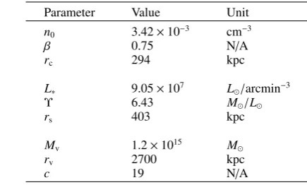
Fig. 2.Profile of the EMOND-calculatedA0(Φ)/a0as a function of clus-ter radius. The blue dashed line is theq=2 model, and the red solid line is theq=1 model. Theq=1 model produces a shallower transi-tion from high to lowA0(Φ) and a smaller magnitude ofA0(Φ) than the q=2 model (see Eq. (6)). We only show radii>100 kpc as this is the important range for the UDGs.
found that EMOND had mixed success in describing the 12 clus-ters from Vikhlinin et al.(2006). We note that the Coma clus-ter was not part of this original study. The work in question used a different baryonic mass profile for both the gas and the galaxies. This result suggests that the EMOND modelling of Hodson & Zhao (2017) might be improved by invoking a dif-ferent functional form for the baryonic mass profile.
Now that we have derived the EMOND mass profile of the Coma cluster, we can make a plot ofA0(Φ) vs radius to show how the EMOND acceleration scale varies in the cluster environment. We show this in Fig.2.
From Fig.2, it is clear that theq=1 model creates a gentler transition of A0(Φ) from the outside of the cluster to the cen-tre than the q = 2 model. It is also clear that the magnitude of A0(Φ) that theq =1 model predicts is much lower than the q = 2 model. This is due in part to the gentler transition, but mainly to the choice ofΦ0, which stopsA0(Φ) reachingA0 max. We describe the effect of this in the following sections.
4. UDG properties
A note on conventions. Throughout the following sections we refer to several mass quantities that we need to define clearly. The “dynamical” mass of the UDGs is the inferred mass from dynamics, thus is the total mass of the system. In aΛCDM con-text, this would be the mass of the stars plus the mass of the dark matter halo. In MOND/EMOND, this would be the baryons +phantom dark matter. The baryonic mass is the to-tal visible mass contained within the UDGs, which we as-sume to be entirely composed of stars and which is determined from the colour-stellar mass relations outlined in Sect.4.2. Fi-nally, the MOND/EMOND mass is the predicted baryonic mass determined from the MOND/EMOND Poisson equation. The MOND/EMOND mass should be equivalent to the baryonic mass if no dark matter is required.
When we modelled the UDGs in MOND/EMOND, we took the dynamical mass of the UDG at the effective radius and determined the MOND/EMOND mass at that radius us-ing the MOND/EMOND recipe. We then compared this to the baryonic mass of these galaxies. Therefore, we need to deter-mine both the dynamical and the baryonic mass for these sys-tems. To do this, we followed the techniques used inZaritsky (2017) and Zaritsky et al. (2008) for the dynamical mass and van Dokkum et al.(2015) for the baryonic mass. We outline the techniques used in these works below.
4.1. Dynamical mass
The dynamical mass of the UDGs is determined from the veloc-ity dispersion and effective radius, assuming virial equilibrium and spherical symmetry, via the formulaWolf et al.(2010; also see Eq. (1) invan Dokkum et al. 2016)
Mdyn|r
s=43re ≈3σ
2rs/G=9.3×105σ2re, (12) where Mdyn(<rs) is the total enclosed dynamical mass at the spherical half-mass radiusrs ≈ 43re, where there is the usual effective radius, that is, the projected circularised half-light ra-dius,σis the velocity dispersion in km s−1 andre is the eff ec-tive 2D radius in kpc. The effective radius was determined and corrected for ellipticity for 46 UDGs within the Coma cluster, and these radii are given invan Dokkum et al.(2015). Currently, there is only one UDGs (Dragonfly 44 (DF44)) in the Coma cluster that has a measured value for the velocity dispersion. We note that the full sample fromvan Dokkum et al.(2015) has 47 objects, but 1 object has incomplete data in the table and thus we disregard this entry. To estimate velocity dispersions for all 46 galaxies in the Coma cluster sample, some assumptions have to be made.
We took a slightly different approach for our study than did Zaritsky(2017).Zaritsky(2017) determined the velocity disper-sions for the UDGs in the Coma cluster by making use of the fundamental manifold (FM). This relation links effective radius, mean surface brightness within the effective 2D radius, and the internal kinematics of the system in question via a nearly power-law-like relation,
logΥe=0.24 logV 2+
0.12 logIe 2
−0.32 logV−0.83 logIe−0.02 log (V Ie)+1.49,(13) whereΥeis the mass-to-light ratio,Ieis the mean surface bright-ness withinre, andV describes the kinematics of the system, mainly the velocity dispersion and rotation, such that V ≡
pσ2 +v2
[image:4.595.68.265.368.488.2]the known relation logre=2 logV−logIe−logΥe−C, which is derived from Eq. (12), to determineVandΥe.Zaritsky(2017) then assumed thatV ≈σ. This value of the velocity dispersion was then corrected via logσcorr =(logσ−0.061)/0.833 to ac-count for a“slight systematic deviation from the expectation”. ThereforeZaritsky(2017) were able to obtain estimates for the velocity dispersions and thus dynamical masses for the UDGs.
When we use the FM relation from a previous study by Zaritsky et al. (2008), there exists a relationship between Ie, re, and σ, without having to solve the system of equations in Zaritsky(2017),
logre=−α2FMlog2σ+(2+2αFMβFM) logσ+BFMlogIe+CFM. (14) In this equation, αFM, βFM, BFM, and CFM are constants that are empirically determined, taking values (Eq. (8) and Fig. 11 from Zaritsky et al. 2006b)α2
FM ≈ 0.63, 2+2αFMβFM ≈ 3.7, BFM ≈ −0.705 and CFM ≈ −2.75. We can use Eq. (14) to find the velocity dispersion analytically using the data given in van Dokkum et al. (2015). The only other difference between our method and that ofZaritsky(2017) is that we did not make the correction to the velocity dispersion and assumed, for now, that all the UDGs lie on the FM. The FM line in Fig. 11 of Zaritsky et al.(2006b) seems to align well with the data points, hence we do not make a correction. We discuss the implications of this later.
The final discussion point is to convert the data table in van Dokkum et al. (2015) into the correct units for the fun-damental manifold equation. The funfun-damental manifold has a 2D effective radius in units of kpc and a mean surface brightness in units of L/pc2. To determine the correct radius, we need to take the radii in Col. 5 (which is the major-axis radius) of the table invan Dokkum et al.(2015) and multiply it by the square root of the axis ratio, given in Col. 7 of the table. For the sur-face brightness, we need to use a standard conversion to change the central surface brightness, given in Col. 4 of the table in van Dokkum et al.(2015) in mag/arcsec2, into the mean surface brightness within an effective radius inL/pc2. This is done by loghIei=−I0+1.822−0.699−M−21.572
2.5 , (15)
where in this case, M is the solar magnitude in the given band, hIei is the mean surface brightness within an effective radius in L/pc2, and I0 is the central surface brightness in mag/arcsec2. See Appendix A for the derivation of Eq. (15). The given formula for converting the surface brightness can be more general depending on the S´ersic index of the modelling. As van Dokkum et al.(2015) used a S´ersic value of 1 for all UDGs, the above formula is valid for all the galaxies in our sample.
After we applied these conversions, we used Eq. (14) to de-termine the estimated velocity dispersion for each UDG and used Eq. (12) to determine the enclosed mass within the 3D radius.
4.2. Estimating the baryonic mass at the effective radius
In the following sections we outline how we inferred the pre-dicted MOND/EMOND mass of the UDGs from the dynamical mass estimate described above. Therefore, to test the validity of the MOND/EMOND formula, we required the approximate en-closed baryonic mass at the effective radius for each UDG in the Coma cluster, which we assumed to be just the inferred stel-lar mass. In order to do this, we followed the technique used in
0 10 20 30 40
0 500 1000 1500 2000 2500
Sample Number
dUDG
-Coma
(
kpc
[image:5.595.316.547.77.224.2])
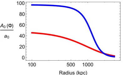
Fig. 3.Minimum projected distance between the centre of the Coma cluster and the UDGs in kpc. The average distance is approximately 1300 kpc. Note that this is the projected distance and the true 3D dis-tance will be higher than this.
van Dokkum et al.(2015). This work takes advantage of the rela-tion between colour and mass-to-light ratio, used inTaylor et al. (2011), which describes a link between the (g−i) colour and the stellar mass-to-light ratio in theiband,
log10M?/M=1.15+0.7(g−i)−0.4Mi, (16) whereMiis the absolute magnitude in theiband andMis the solar mass, not to be confused with the solar magnitude used previously. We note that inTaylor et al. (2011) the stellar pop-ulations were modelled using a canonical initial mass function (IMF;Chabrier 2003;Kroupa 2001;Kroupa et al. 2013). From this, we calculated the stellar mass using only colour and magni-tude. Theg-band magnitude is given for 46 UDGs in the Coma cluster invan Dokkum et al.(2015). For the sample, the average g−icolour ishg−ii ≈0.8±0.1. This is the value we adopted for each UDG. Therefore thei-band magnitude can be calculated from the quotedg-band magnitude viaMi≈Mg−0.8. We there-fore have all the necessary quantities to derive a stellar mass for the UDGs. We note that the mass calculated via Eq. (16) is the total stellar mass. The stellar mass withinrs, which is what we are interested in, is half ofM?.
4.3. Distance from the centre of the cluster
As we only have the 2D projected map of the Coma cluster and the UDGs, it is not possible to derive their exact radii from the centre of the cluster. We can calculate the minimum radius at which the UDGs should be from the right ascension and dec-lination of the UDGs, however, as given in van Dokkum et al. (2015). If we assume that all the UDGs lie at the same distance as the Coma cluster itself, we can find their minimum distance from
dUDG−Coma≈dComaθUDG−Coma, (17) wheredComais the distance to the Coma cluster andθUDG−Coma is the angular separation in radians between the UDG and the Coma cluster centre.
5. MOND and EMOND modelling
In this section we describe how the UDGs were modelled in the regular MOND and EMOND paradigms. To do this, we took the dynamical mass, derived from the predicted ve-locity dispersions (Sect. 4.1), and substituted the value into the MOND (and EMOND) formula. From this, we deter-mined the MOND/EMOND mass, which is required to sat-isfy the MOND/EMOND equations. Assuming that the galaxy is dominated by stellar mass, we then compared this MOND/ EMOND mass to the baryonic mass derived in Sect.4. If the MOND/EMOND paradigm is correct, these two methods should be consistent. All this modelling was conducted under the as-sumption that the UDGs are spherical and in dynamical equilib-rium. We note that the averageb/aratio for the sample is 0.74.
5.1. MOND
To begin the MOND modelling, we started by assuming that the UDGs are isolated systems. If they are isolated, we can use the simple spherical MOND relation to model them,
∇ΦMOND=µ ∇Φdyn
a0 !
∇Φdyn, (18)
where ∇ΦMOND is the MOND-predicted baryonic mass and
∇Φdyn = GMdyn(r)/r2 is the dynamical acceleration. As dis-cussed, we can then find the MOND mass from the calculated dynamical mass of the UDGs.
However, this is not the correct picture as UDGs are not isolated, they are within the external field of the cluster. The MOND formula has to be modified to take into consideration the external field of the cluster (e.g. Bekenstein & Milgrom 1984; Famaey et al. 2007;Wu et al. 2008;Haghi et al. 2016),
p
(∇ΦMOND)2+(∇Φ
MOND ext)2≈ µ q
(∇Φdyn)2+(∇Φext)2 a0 q
(∇Φdyn)2+(∇Φext)2. (19)
The results are found to be nearly the same when we assume thata andgextare orthogonal. Assuming that the external field is entirely dominated by the Coma cluster, we determined the magnitude of the external field from our model of the Coma cluster in Sect. 3. The external field used for each UDG was determined from the distance it lies away from the centre of the cluster, which we calculated in Sect.4.3.
We expect that the external field increases the overall accel-eration across the UDGs, pushing the internal dynamics closer to Newtonian as the MOND interpolation function argument is increased. This highlights the tension between the MOND paradigm and the UDG observations. Although we repeat that this modelling assumes equilibrium and sphericity. Relaxing this may yield less tension in the MOND framework.
5.2. EMOND
As we have seen in our Coma cluster EMOND model, the eff ec-tive value ofa0 is increased within the cluster. This could raise the dark matter-like effects within the UDGs even with the ex-ternal field of the cluster dominating the dynamics. This is due to the so-called external potential effect. As the UDGs are in the deep potential well of the Coma cluster, under the prediction of
the EMOND paradigm, the internal dynamics of the UDGs are affected. The modified version of Eq. (19) for EMOND is
p
(∇ΦEMOND)2+(∇ΦEMOND ext)2
≈µ q
(∇Φdyn)2+(∇Φ ext)2 A0
Φdyn+ Φext q
(∇Φdyn)2+(∇Φ
ext)2. (20)
Making the assumption that A0(Φ) is approximately constant across the UDGs as they are so small, we can rewrite Eq. (20) as
(∇ΦEMOND)2 =µ p
(∇Φ)2+(∇Φ ext)2 A0(Φext)
2
(∇Φ)2+(∇Φext)2
−µ ∇Φext
A0(Φext) !2
∇Φ2ext, (21) where we have eliminated ∇ΦEMOND ext from Eq. (20) via
∇ΦEMOND ext=µ ∇Φ
ext
A0(Φext)
∇Φext. Although the gravitational po-tential of the Coma clusters dominates the UDGs in our model, the gravitational accelerations of the UDGs are still relevant and thus we do not neglect them.
To highlight the meaning of the different mass symbols, if the MOND paradigm is correct,∇ΦMOND should be equivalent to the acceleration from the baryons,∇Φb≡GL∗/r2 (M/L∗). In galaxy clusters, if no dark matter is present,∇ΦMOND > ∇Φb. The hope is that the EMOND formalism can fix this such that
∇ΦEMOND ≈ ∇Φb (within modelling and data errors). In galax-ies, as MOND should be a limit of EMOND, we should have the relation∇ΦEMOND=∇ΦMOND≈ ∇Φb.
Equations (18), (19), and (21) can then be used to calculate the predicted MOND/EMOND mass of the UDGs given the dy-namical mass of the UDGs and the external field and potential, which is derived from the fundamental manifold (see Sect.4.1) and the Coma model, respectively.
6. Results
For our results, we did not perform a rigorous error analysis as there are many sources of errors from all the measurements and modelling of the UDGs as well as scatter from the FM and the model of the Coma cluster. We aim to determine whether EMOND is a possible explanation for the UDG over-massive dark haloes.
In the following plots we show the ratio of the predicted by the MOND/EMOND mass and the baryonic mass calculated from the colour. Ideally, this ratio should be 1. If the ratio is lower than 1, either the MOND/EMOND paradigm predicts that there should be less mass than is permitted by the stellar mass estimates, or the stellar mass estimate is too high. If the ratio is higher than 1, the MOND formulation predicts that there should be more mass present than is permitted by the stellar mass esti-mates, or the stellar mass estimates are too low. This conclusion rests heavily on the assumption that the dynamical mass esti-mates for the UDGs are correct, which they may not be.
We begin by showing the result for a MOND model with no effects from the Coma cluster (Fig.4). We see that for a regu-lar MOND model, the overall trend seems to be that the ratio is lower than 1 by a factor of approximately 2. Therefore, per-haps within the errors, MOND with no external field might be sufficient in explaining the UDG masses.
0 500 1000 1500 2000 2500 0.0
0.2 0.4 0.6 0.8 1.0
DUDG-Coma(kpc)
MMOND
/
M
[image:7.595.316.546.79.394.2]b
Fig. 4.Ratio of the MOND mass to the estimated stellar mass from colour as a function of the distance to the cluster centre. No effect from the Coma cluster is considered.
0 500 1000 1500 2000 2500
0 2 4 6 8 10 12 14
DUDG-Coma (kpc)
MMOND
/
M
b
Fig. 5.Same as Fig.4, except that we include the external field from the Coma cluster. The MOND mass is much higher than the colour-predicted stellar mass.
the UDGs, increasing the argument in the MOND interpola-tion funcinterpola-tion, and thus driving the systems closer to Newtonian physics. We therefore see that including the external field makes the MOND model a poorer fit, the ratio is higher than 1, therefore requiring much more stellar mass than is available according to the colour estimate.
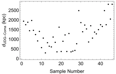
We then show how the EMOND effect of increasing a0 across the UDGs changes the result (Fig. 6). We find that the EMOND prediction improves the MOND fit substantially within the expected errors. We also note that theq=2 model (top panel) seems to produce a trend such that the farther out the UDG, the higher the predicted EMOND mass from the EMOND formal-ism compared to the stellar mass. This is less of an issue with the q =1 model, demonstrating that the UDGs provide a stringent constraint in the allowed functional form ofA0(Φ). This might be an indication that rigorous numerical testing and a larger sample of UDGs might find that further refining the EMOND parame-ters and interpolation function might produce an even better fit. This is beyond the scope of this paper. Another point of note is the fact that the outer UDG values are similar in the MOND and EMOND case. The reason is that the EMOND formalism asymptotically tends to MOND in the outer part of the cluster, as desired.
The above results seem to show that when we take the dy-namical mass of the UDGs, the stellar mass of the UDGs, the EMOND function, and the model of the Coma cluster at face
0 500 1000 1500 2000 2500
0.0 0.5 1.0 1.5 2.0 2.5 3.0
DUDG-Coma (kpc)
MEMOND
/
M
b
0 500 1000 1500 2000 2500
0.0 0.5 1.0 1.5 2.0 2.5 3.0
DUDG-Coma (kpc)
MEMOND
/
M
[image:7.595.52.283.79.235.2]b
Fig. 6. Same as Fig. 5, except with the EMOND correction to the MOND acceleration scale. Thetop panelshows theq=2 model and the bottom paneltheq=1 model (see Eq. (6)). The EMOND paradigm pre-dicts a reasonable EMOND mass for the UDG sample in both models. Theq=2 model shows that the required mass-to-light ratio increases with distance, which is an undesirable feature. Theq=1 model shows that a constant mass-to-light ratio with distance is a good fit to the data, which seems more plausible.
value, EMOND is able to explain the Coma cluster mass profile and the UDGs within it. Theq = 1 model produces a better fit to the data than theq = 2 model in terms of how the distance of the UDGs from the centre of the Coma cluster is affected by EMOND.
There will undoubtedly be sources of errors within these cal-culations from spherical symmetry assumptions, scatter around the FM, the error in the Coma cluster mass model, etc. that will alter the result. The main source of error is most likely the uncertainty in the stellar mass-to-light ratio and the use of the M/L−(g−i) relation.
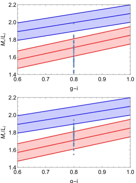
[image:7.595.53.280.284.440.2]0.6 0.7 0.8 0.9 1.0 1.4
1.6 1.8 2.0 2.2
g-i M*
/
Li
0.6 0.7 0.8 0.9 1.0
1.4 1.6 1.8 2.0 2.2
g-i M*
/
[image:8.595.52.280.77.383.2]Li
Fig. 7.Stellar mass-to-light functions fromTaylor et al.(2011; red) and Bell et al.(2003; blue) as a function ofg−icolour. We show approxi-mate error bars of 0.1 dex for each case. Thetop panelshows the results for theq=2 model, and thebottom panelshows theq=1 model (see Eq. (6)). The blue dots show where the UDGs must lie assuming that the EMOND formulation is correct. This shows that it may be possible for most of the UDGs to be explained by EMOND within the range of stellar mass-to-light ratio allowed. Theq=1 model again shows better results.
Fig.7. We recall at this point that the 0.8 value is an average with an error of±0.1, therefore there is an extra source of uncertainty. Figure7shows that there seems to be a very large scope for error in the mass-to-light ratio of the stars in the UDG, within which most UDGs in our sample lie. We can therefore con-clude that adjusting the stellar mass-to-light ratio can explain the UDGs mass, within the error bars, assuming that the EMOND modelling of the UDGs is valid.
7. Adjusting the EMOND formulation
The above results show that theq=1 model explains the UDGs better than the q = 2 model used inHodson & Zhao (2017). For completeness, we therefore need to repeat the analysis of Hodson & Zhao(2017) to confirm that theq =1 model is con-sistent with the cluster sample ofVikhlinin et al.(2006). To do this, we briefly review the Hodson & Zhao (2017) work and recreate their Figs. 17–22 with the updated function forA0(Φ).
One method of testing modified gravity theories is by com-paring the estimated “total” mass, calculated from dΦ/dr r2/G, whereΦis the total gravitational potential derived from the Pois-son equation, and the mass calculated by assuming the intra-cluster gas is in hydrostatic equilibrium, which we call the dy-namical mass. The expression for dydy-namical mass, assuming Newtonian physics, is determined by solving the equation of
hydrostatic equilibrium, Mdyn(r)=−
kT(r)r Gwmp
"dlnρ g(r) dlnr +
dlnT(r) dlnr
#
, (22)
whereρg(r) is the density of the gas, T(r) is the temperature of the gas,kis the Boltzmann constant,mp is the proton mass, and w is the mean molecular weight. Therefore, for a given gas density and temperature, the dynamical mass can be calcu-lated. In theory, the dynamical mass should be comparable to dΦ/dr r2/G. In regular MOND, dΦ/dr r2/Gis much lower than the dynamical mass in galaxy clusters. The original motivation for formulating EMOND was to rectify this discrepancy. This was the goal ofHodson & Zhao(2017).
As EMOND is sensitive to the magnitude of the gravitational potential, to solve the EMOND Poisson equation, a boundary potential had to be defined (Hodson & Zhao 2017). To estimate this quantity,Hodson & Zhao(2017) used the analytical best-fit Navarro-Frenk-White (NFW) profiles for each cluster and as-sumed thatΦ(rout)≈ΦNFW(rout),whereroutwas defined as some boundary outside the cluster. They then showed the range of solutions from Φ(rout) = (0.5−1.5) ×ΦNFW(rout) to obtain an idea of how changing the boundary potential affected the re-sult. To be consistent, we here set the boundary potential at the virial radius for each cluster to take the same value as was used for the Coma cluster. We also show the boundary potential for Φ(rv)=(0.9−1.1)×Φ(rv) in contrast to the previous work. Al-though we have treated the boundary potential as a free param-eter, we hope that in the future, when the EMOND theory has a covariant form, matching the non-linear regime onto the cos-mological solution will fix this value for each cluster. Therefore the boundary potential will be determined from the theory and not left as a free parameter. This is beyond current EMOND ca-pabilities, and thus we have set all boundary potentials to be the same for each cluster. In defense of this approximations, we ex-pect that clusters of similar masses should lie in similar poten-tial wells.
For the baryonic mass model for these galaxies, the gas was modelled as inVikhlinin et al.(2006),Hodson & Zhao(2017). We did change the contribution of the galaxies, however, to have a similar mass profile as the Coma cluster. We note that each cluster will in practice have a different mass contribution from the galaxies. We did not attempt to find the best-fit galaxy model for each cluster. This is best left until the theory of EMOND is clearer, specifically with regard to understanding the boundary potential.
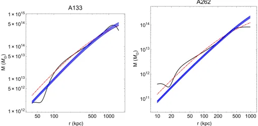
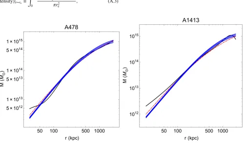
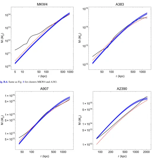
Repeating the above steps for the new A0(Φ) function, we show the updated mass plots for the cluster sample (Figs. 8, B.1−B.5).
50 100 500 1000 1×10¹²
5×10¹²
1×10¹³
5×10¹³
1×10¹⁴
5×10¹⁴
1×10¹⁵
r(kpc)
M
(
M⊙
)
A133
10 20 50 100 200 500 1000 1011
1012
1013
1014
r(kpc)
M
(
M⊙
)
[image:9.595.40.552.82.333.2]A262
Fig. 8.Recreated Figs. 17–22 fromHodson & Zhao(2017) with the modifiedA0(Φ) function found under the UDG constraints. The red dashed line shows the best-fitΛCDM model fromVikhlinin et al.(2006), the black line the dynamical mass derived from Eq. (22), and the blue shaded region shows the EMOND-predicted mass. Here we show clusters A133 and A262.
of the interpolation function is still consistent with the previous EMOND work.
8. Discrepancy with observations
Although our above analysis has shown consistency between the Coma cluster and UDGs masses under the EMOND paradigm, we have made some rather large assumptions, the main assump-tion being that the FM can be used to determine the veloc-ity dispersion of the UDGs. If we take the estimate for DF44, which is the only UDG in the sample that has been observed (≈47+8
−6 km s
−1), the FM under-predicts the velocity dispersion by a factor of ≈2.7 (the FM-predicted velocity dispersion for DF44 is≈17.4 km s−1). If we then take the published observed data fromvan Dokkum et al.(2016), EMOND would predict a baryonic mass of≈7.7×10⁸Mand thus the ratio between this EMOND (q = 1 model) mass and the baryonic mass is≈7.5, which is quite a substantial difference. This result is improved if the EMOND boundary potential chosen for the Coma clus-ter is increased. Choosing the boundary to be 3.5×10¹²m2s−2, the ratio is reduced to ≈6. When we chose this potential and took the lowest bound for the velocity dispersion (41 km s−1), the ratio further decreased to ≈4.5. This could be further im-proved by choosing a higher stellar mass-to-light ratio than is used invan Dokkum et al.(2016). However, it must be checked which values for the boundary potential are allowed by the data for Coma. This would require further work, which is beyond the scope of this paper.
The reason that our UDG dynamical masses differ from the work ofZaritsky(2017) is that these authors corrected the veloc-ity dispersion that is due to the discrepancy between the observed velocity dispersion and the FM estimated value (see Fig. 1 of Zaritsky 2017). In our analysis, we used a different form of the FM. The source of the discrepancy needs to be investigated in further work.
More detailed observations of more UDGs in the Coma clus-ter are required to declus-termine whether the over-massive dark halo of DF44 is a statistical outlier in the sample or if the interpre-tation of the FM used in our work disagrees with the current observations. A deeper understanding of UDG properties may arise from studying tidal effects from the cluster and/or compar-ing formation scenarios with that of remnant systems, such as those described byKroupa(1997).
9. Conclusion
We modelled the Coma cluster in the EMOND paradigm and compared the predicted enclosed mass profile to that of a pure Newtonian model. We found that the EMOND result bears an extraordinary resemblance to the DM profile used in Łokas & Mamon(2003). This is quite a successful result for the EMOND paradigm. The success of this result warrants further study of EMOND, taking into careful consideration the func-tional form of the baryonic mass profile and the boundary poten-tial used to solve the Poisson equation.
We then moved on to make a model of UDGs in EMOND. We used this to determine the MOND/EMOND mass required to satisfy the MOND/EMOND formula. We then compared this to the baryonic mass, in the form of stars, that is predicted by the UDG galaxy colour.
However, the results of this work disagree with observations of UDG DF44. A reanalysis of this calculation must be con-ducted when more UDG velocity dispersions are observed.
The UDGs serve as a very good test for MOND-like grav-ity theories and should be studied in more detail. The next step is to conduct the same analysis for the Virgo cluster and its UDG population.
UDGs are still a relatively new discovery, with limited ob-servations and a small sample size. More measurements of the velocity dispersions for the UDGs would produce more accurate dynamical mass estimates. It is hard to discuss possible forma-tion scenarios in the context of EMOND as it is still a relatively new theory on which limited research has been conducted. We have shown that a possible solution to the mass discrepancy in galaxy clusters in a MOND-like paradigm, EMOND, may also hold the answer to the nature of these UDGs. When two prob-lems have one solution, it warrants further investigation, and we hope that EMOND will be investigated further as a result of this.
Acknowledgements. We would like to thank Anne-Marie Weijmans and Benoit Famaey for general comments on the draft. We would also like to thank Dennis Zaritsky for discussions on the fundamental manifold. We must also thank the anonymous referee whose comments were both welcomed and valued. A.O.H. is supported by Science and Technologies Funding Council (STFC) studentship (Grant code: 1-APAA-STFC12).
References
Angus, G. W. 2009,MNRAS, 394, 527
Angus, G. W., & Diaferio, A. 2011,MNRAS, 417, 941
Angus, G. W., Famaey, B., & Buote, D. A. 2008,MNRAS, 387, 1470 Angus, G. W., Diaferio, A., Famaey, B., & van der Heyden, K. J. 2013,MNRAS,
436, 202
Beasley, M. A., Romanowsky, A. J., Pota, V., et al. 2016,ApJ, 819, L20 Bekenstein, J., & Milgrom, M. 1984,ApJ, 286, 7
Bell, E. F., McIntosh, D. H., Katz, N., & Weinberg, M. D. 2003,ApJS, 149, 289 Blanchet, L., & Novak, J. 2011,MNRAS, 412, 2530
Boylan-Kolchin, M., Bullock, J. S., & Kaplinghat, M. 2011,MNRAS, 415, L40 Boylan-Kolchin, M., Bullock, J. S., & Kaplinghat, M. 2012,MNRAS, 422, 1203 Chabrier, G. 2003,ApJ, 586, L133
Derakhshani, K., & Haghi, H. 2014,ApJ, 785, 166 Djorgovski, S., & Davis, M. 1987,ApJ, 313, 59
Donato, F., Gentile, G., Salucci, P., et al. 2009,MNRAS, 397, 1169 Dressler, A., Lynden-Bell, D., Burstein, D., et al. 1987,ApJ, 313, 42
Dubinski, J., & Carlberg, R. G. 1991,ApJ, 378, 496 Famaey, B., & Binney, J. 2005,MNRAS, 363, 603 Famaey, B., & McGaugh, S. S. 2012,Liv. Rev. Rel., 15, 10 Famaey, B., Bruneton, J.-P., & Zhao, H. 2007,MNRAS, 377, L79 Graham, A. W., & Driver, S. P. 2005,PASA, 22, 118
Haghi, H., Bazkiaei, A. E., Zonoozi, A. H., & Roupa, P. 2016,MNRAS, 458, 4172
Hodson, A., & Zhao, H. 2017,A&A, 598, A127
Ibata, R. A., Lewis, G. F., Conn, A. R., et al. 2013,Nature, 493, 62 Klypin, A., Kravtsov, A. V., Valenzuela, O., & Prada, F. 1999,ApJ, 522, 82 Koda, J., Yagi, M., Yamanoi, H., & Komiyama, Y. 2015,ApJ, 807, L2 Kroupa, P. 1997,New Astron., 2, 139
Kroupa, P. 2001,MNRAS, 322, 231 Kroupa, P. 2012,PASA, 29, 395 Kroupa, P. 2015,Can. J. Phys., 93, 169
Kroupa, P., Famaey, B., de Boer, K. S., et al. 2010,A&A, 523, A32
Kroupa, P., Weidner, C., Pflamm-Altenburg, J., et al. 2013, The Stellar and Sub-Stellar Initial Mass Function of Simple and Composite Populations, eds. T. D. Oswalt, & G. Gilmore (Dordrecht: Springer Science+Business Media), 115 Łokas, E. L., & Mamon, G. A. 2003,MNRAS, 343, 401
Mihos, J. C., Durrell, P. R., Ferrarese, L., et al. 2015,ApJ, 809, L21 Milgrom, M. 1983a,ApJ, 270, 371
Milgrom, M. 1983b,ApJ, 270, 384 Milgrom, M. 1983c,ApJ, 270, 365 Milgrom, M. 2014,Scholarpedia, 9, 31410
Moore, B., Ghigna, S., Governato, F., et al. 1999,ApJ, 524, L19
Pawlowski, M. S., Famaey, B., Merritt, D., & Kroupa, P. 2015,ApJ, 815, 19 Roman, J., & Trujillo, I. 2017,MNRAS, 468, 703
Sanders, R. H. 1999,ApJ, 512, L23 Sanders, R. H. 2003,MNRAS, 342, 901
Taylor, E. N., Hopkins, A. M., Baldry, I. K., et al. 2011,MNRAS, 418, 1587 van Dokkum, P. G., Abraham, R., Merritt, A., et al. 2015,ApJ, 798, L45 van Dokkum, P., Abraham, R., Brodie, J., et al. 2016,ApJ, 828, L6 Vikhlinin, A., Kravtsov, A., Forman, W., et al. 2006,ApJ, 640, 691 Walker, M. G., & Peñarrubia, J. 2011,ApJ, 742, 20
Wolf, J., Martinez, G. D., Bullock, J. S., et al. 2010,MNRAS, 406, 1220 Wu, X., & Kroupa, P. 2013,MNRAS, 435, 728
Wu, X., & Kroupa, P. 2015,MNRAS, 446, 330
Wu, X., Famaey, B., Gentile, G., Perets, H., & Zhao, H. 2008,MNRAS, 386, 2199
Zaritsky, D. 2017,MNRAS, 464, L110
Zaritsky, D., Gonzalez, A. H., & Zabludoff, A. I. 2006a,ApJ, 642, L37 Zaritsky, D., Gonzalez, A. H., & Zabludoff, A. I. 2006b,ApJ, 638, 725 Zaritsky, D., Zabludoff, A. I., & Gonzalez, A. H. 2008, in Formation and
Evolution of Galaxy Disks, eds. J. G. Funes, & E. M. Corsini,ASP Conf. Ser., 396, 381
Appendix A: Surface brightness conversion
van Dokkum et al. (2015) provided the central surface bright-ness. The FM required the mean surface brightness at the eff ec-tive radius. Converting the surface brightness from the value at the centre of the UDG into the mean surface brightness at the ef-fective radius is a simple and standard calculation that we review here for completeness. For a full more detailed look at the calcu-lation, we refer toGraham & Driver(2005), where most of the equations below come from. Light profiles are commonly mod-elled with a S´ersic profile. In terms of the surface brightness,I, the S´ersic profile is
I(r)=Ie+2.5bn ln 10
r re
!1/n
−1
, (A.1)
wherenparametrises the S´ersic index that describes the shape of the profile, andbnis a constant that is defined for eachn. As
van Dokkum et al.(2015) quoted the central surface brightness and the FM requires the mean surface brightness at the effective radius, the first step is to solve Eq. (A.1) forIe. All the UDGs in the sample were modelled with a S´ersic index n = 1. The correspondingb1value is≈1.678. Therefore
Ie≈I0+1.821. (A.2)
Next we transformed this value into the average value at the ef-fective radius. The average intensity is defined to be
hIntensityi|r=re ≡
Z re
0
Intensity(r) 2πrdr πre2
, (A.3)
where the intensity can be transformed into surface brightness viaI=2.5 log10(intensity). Solving Eq. (A.3) and moving from intensity to surface brightness, we obtain
hIei=Ie−2.5 log10 "
nexp(bn) b2n
n
Γ(2n) #
. (A.4)
Inserting the numbers, we arrive at
hIei=I0+1.821−0.699, (A.5)
where we have expressed the value in terms of the central value of surface brightness. Currently, the mean surface brightness is in units of mag/arcsec2, which we need to convert intoL/pc2. This is done via
I(L/pc2)=exp "
−(I(mag/arcsec
2)−M
−21.572) 2.5
#
, (A.6)
whereMis the solar magnitude in the given band. Therefore,
hIei(L/pc2)=exp "
−I0+1.821−0.699M−21.572
2.5
#
, (A.7)
whereI0is in mag/arcsec2. This is the derivation of Eq. (15).
Appendix B: Additional figures
50 100 500 1000
5×10¹² 1×10¹³ 5×10¹³ 1×10¹⁴ 5×10¹⁴ 1×10¹⁵
r(kpc)
M
(
M⊙
)
A478
50 100 500 1000 1012
1013
1014
1015
r(kpc)
M
(
M⊙
)
[image:11.595.49.548.397.691.2]A1413
50 100 500 1000
1×10¹²
5×10¹²
1×10¹³
5×10¹³
1×10¹⁴
5×10¹⁴
1×10¹⁵
r(kpc)
M
(
M⊙
)
A1795
10 50 100 500 1000
1011
1012
1013
1014
r(kpc)
M
(
M⊙
)
[image:12.595.43.557.79.627.2]A1991
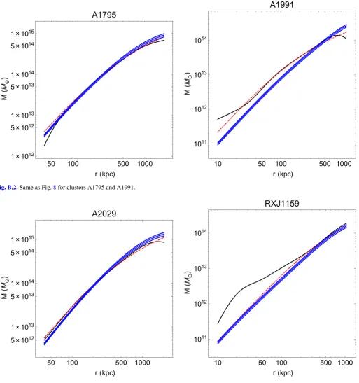
Fig. B.2.Same as Fig.8for clusters A1795 and A1991.
50 100 500 1000
5×10¹²
1×10¹³
5×10¹³
1×10¹⁴
5×10¹⁴
1×10¹⁵
r(kpc)
M
(
M⊙
)
A2029
10 50 100 500 1000
1011
1012
1013
1014
r(kpc)
M
(
M⊙
)
[image:12.595.46.325.94.333.2]RXJ1159
5 10 50 100 500 1000
1010
1011
1012
1013
1014
r(kpc)
M
(
M⊙
)
MKW4
50 100 500 1000
1012
1013
1014
1015
r(kpc)
M
(
M⊙
)
[image:13.595.42.559.71.604.2]A383
Fig. B.4.Same as Fig.8for clusters MKW4 and A383.
50 100 500 1000
5×10¹²
1×10¹³
5×10¹³
1×10¹⁴
5×10¹⁴
1×10¹⁵
r(kpc)
M
(
M⊙
)
A907
100 200 500 1000 2000
1×10¹³
5×10¹³
1×10¹⁴
5×10¹⁴
1×10¹⁵
r(kpc)
M
(
M⊙
)