Variation in stem mortality rates determines patterns of
above-ground biomass in Amazonian forests:
implications for dynamic global vegetation models
M I C H E L L E O . J O H N S O N1, D A V I D G A L B R A I T H1, M A N U E L G L O O R1,H A N N E S D E D E U R W A E R D E R2, M A T T H I E U G U I M B E R T E A U3 , 4, A N J A R A M M I G5 , 6, K I R S T E N T H O N I C K E6, H A N S V E R B E E C K2, C E L S O V O N R A N D O W7,
A B E L M O N T E A G U D O8, O L I V E R L . P H I L L I P S1, R O E L J . W . B R I E N E N1, T E D R . F E L D P A U S C H9, G A B R I E L A L O P E Z G O N Z A L E Z1, S O P H I E F A U S E T1, C A R L O S A . Q U E S A D A1 0, B R A D L E Y C H R I S T O F F E R S E N1 1 , 1 2, P H I L I P P E C I A I S3, G I L V A N S A M P A I O7, B A R T K R U I J T1 3, P A T R I C K M E I R1 1 , 1 4, P A U L M O O R C R O F T1 5,
K E Z H A N G1 6, E S T E B A N A L V A R E Z - D A V I L A1 7, A T I L A A L V E S D E O L I V E I R A1 0, I E D A
A M A R A L1 0, A N A A N D R A D E1 0, L U I Z E . O . C . A R A G A O8, A L E J A N D R O A R A U J O
-M U R A K A -M I1 8, E R I C J . M . M . A R E T S1 3, L U Z M I L A A R R O Y O1 8, G E R A R D O A . A Y M A R D1 9,
C H R I S T O P H E R B A R A L O T O2 0, J O C E L Y B A R R O S O2 1, D A M I E N B O N A L2 2, R E N E B O O T2 3,
J O S E C A M A R G O1 0, J E R O M E C H A V E2 4, A L V A R O C O G O L L O2 5, F E R N A N D O C O R N E J O V A L V E R D E2 6, A N T O N I O C . L O L A D A C O S T A2 7, A N T H O N Y D I F I O R E2 8, L E A N D R O F E R R E I R A2 9, N I R O H I G U C H I1 0, E U R I D I C E N . H O N O R I O3 0, T I M J . K I L L E E N3 1, S U S A N G . L A U R A N C E3 2, W I L L I A M F . L A U R A N C E3 2, J U A N L I C O N A3 3, T H O M A S L O V E J O Y3 4, Y A D V I N D E R M A L H I3 5, B I A M A R I M O N3 6, B E N H U R M A R I M O N J U N I O R3 6, D A R L E Y C . L . M A T O S2 9, C A S I M I R O M E N D O Z A3 7, D A V I D A . N E I L L3 8, G U I D O P A R D O3 9, M A R I E L O S P E N˜ A - C L A R O S3 3 , 4 0, N I G E L C . A . P I T M A N4 1, L O U R E N S P O O R T E R4 0, A D R I A N A P R I E T O4 2, H I R M A R A M I R E Z - A N G U L O4 3, A N A N D R O O P S I N D4 4, A G U S T I N R U D A S4 2,
R A F A E L P . S A L O M A O2 9, M A R C O S S I L V E I R A4 5, J U L I A N A S T R O P P4 6, H A N S T E R S T E E G E4 7, J O H N T E R B O R G H4 1, R A Q U E L T H O M A S4 4, M A R I S O L T O L E D O3 3,
A R M A N D O T O R R E S - L E Z A M A4 3, G E E R T J E M . F . V A N D E R H E I J D E N4 8,
R O D O L F O V A S Q U E Z9, I M A CEL I A G U I M A R AE S V I E I R A~ 2 9, E M I L I O V I L A N O V A4 3,
V I N C E N T A . V O S4 9 , 5 0 and T I M O T H Y R . B A K E R1 1
School of Geography, University of Leeds, Leeds LS6 2QT, UK,2CAVElab Computational & Applied Vegetation Ecology, Faculty of Bioscience Engineering, Ghent University, Coupure Links 653, B-9000 Gent, Belgium,3Laboratoire des Sciences du Climat et de l’Environnement, LSCE/IPSL, CEA-CNRS-UVSQ, Universite´ Paris-Saclay, F-91191 Gif-sur-Yvette, France,4UMR 7619
METIS, IPSL, Sorbonne Universite´s, UPMC, CNRS, EPHE, 75252 Paris, France,5TUM School of Life Sciences Weihenstephan,
Technical University Munich, Hans-Carl-von-Carlowitz-Platz 2, 85354 Freising, Germany,6Potsdam Institute for Climate Impact
Research (PIK), Telegrafenberg A62, PO Box 60 12 03, D-14412 Potsdam, Germany,7INPE, Av. Dos Astronautas, 1.758, Jd.
Granja, CEP: 12227-010 Sao Jose dos Campos, SP, Brazil,8Jardı´n Bota´nico de Missouri, Prolongacion Bolognesi Mz.e, Lote 6,
Oxapampa, Pasco, Peru,9Geography, College of Life and Environmental Sciences, University of Exeter, Rennes Drive, Exeter EX4
4RJ, UK,10INPA, Av. Andre´ Arau´jo, 2.936, CEP 69067-375 Petro´polis, Manaus, AM, Brazil,11School of Geosciences, University of Edinburgh, Edinburgh EH9 3FF, UK,12Earth and Environmental Sciences Division, Los Alamos National Laboratory, PO Box 1663, Los Alamos, NM 87545, USA,13ALTERRA, Wageningen-UR, PO Box 47, 6700 AA Wageningen, The Netherlands,
14
Research School of Biology, Australian National University, Canberra, ACT 0200, Australia,15Department of Organismic and Evolutionary Biology, Harvard University, 26 Oxford Street, Cambridge, MA 02138, USA,16Cooperative Institute for Mesoscale Meteorological Studies, University of Oklahoma, National Weather Center, Suite 2100, 120 David L. Boren Blvd, Norman, OK 73072, USA,17Fundacio´n Con-Vida, Cr68 A 46 A-77 Medellı´n, Medellı´n, Colombia,18Museo de Historia Natural Noel Kempff Mercado, Universidad Autonoma Gabriel Rene Moreno, Casilla 2489, Av. Irala 565, Santa Cruz, Bolivia,19UNELLEZ-Guanare, Programa de Ciencias del Agro y el Mar, Herbario Universitario (PORT), Mesa de Cavacas, Estado Portuguesa 3350, Venezuela,
20
Department of Biological Sciences, International Center for Tropical Botany (ICTB), Florida International University, 112200 SW 8th Street, OE 167, Miami, FL 33199, USA,21Universidade Federal do Acre, Campus de Cruzeiro do Sul, Rio Branco, Brazil, 22INRA, UMR 1137 “Ecologie et Ecophysiologie Forestiere”, 54280 Champenoux, France,23Tropenbos International, PO Box 232,
6700 AE Wageningen, The Netherlands,24Universite´ Paul Sabatier CNRS, UMR 5174 Evolution et Diversite´ Biologique,
Correspondence: Timothy R. Baker, tel. +44 (0)113 3438352, fax +44 (0)113 343 5259, e-mail: [email protected]
baˆtiment 4R1, 31062 Toulouse, France,25Jardı´n Bota´nico de Medellı´n Joaquı´n Antonio Uribe, Calle 73 # 51 D 14 Medellı´n,
Colombia,26Andes to Amazon Biodiversity Program, Puerto Maldonado, Madre de Dios, Peru´,27Centro de Geociencias,
Universidade Federal do Para, CEP 66017-970 Belem, Para, Brazil,28Department of Anthropology, University of Texas at Austin, SAC Room 5.150, 2201 Speedway Stop C3200, Austin, TX 78712, USA,29Museu Paraense Emilio Goeldi, Av. Magalha˜es Barata, 376 - Sa˜o Braz, CEP: 66040-170 Bele´m, PA, Brazil,30Instituto de Investigaciones de la Amazonı´a Peruana, Av. Jose´ Quin˜ones km 2.5, Iquitos, Peru´,31World Wildlife Fund, 1250 24th St NW, Washington, DC 20037, USA,32Centre for Tropical Environmental and Sustainability Science (TESS) and College of Marine and Environmental Sciences, James Cook University, Cairns, Qld 4878, Australia,33Instituto Boliviano de Investigacio´n Forestal, C.P. 6201 Santa Cruz de la Sierra, Bolivia,34Environmental Science and Policy Department and the Department of Public and International Affairs at George Mason University (GMU), 3351 Fairfax Drive, Arlington, VA 22201, USA,35Environmental Change Institute, School of Geography and the Environment, University of Oxford, South Parks Road, Oxford OX1 3QY, UK,36Universidade do Estado de Mato Grosso, Campus de Nova Xavantina, Caixa Postal 08, CEP 78.690-000 Nova Xavantina, MT, Brazil,37Escuela de Ciencias Forestales (ESFOR), Av. Final Atahuallpa s/n,
Casilla 447, Cochabamba, Bolivia,38Facultad de Ingenierı´a Ambiental, Universidad Estatal Amazo´nica, Paso lateral km 2 1/2 via
Napo, Puyo, Pastaza, Ecuador,39Universidad Autonoma del Beni, Campus Universitario, Av. Eje´rcito Nacional, final, Riberalta,
Beni, Bolivia,40Forest Ecology and Forest Management Group, Wageningen University, PO Box 47, Wageningen 6700 AA, The
Netherlands,41Center for Tropical Conservation, Duke University, Box 90381, Durham, NC 27708, USA,42Doctorado Instituto
de Ciencias Naturales, Universidad Nacional de Colombia, Bogota´, Colombia,43Instituto de Investigaciones para el Desarrollo
Forestal, Universidad de Los Andes, Avenida Principal Chorros de Milla, Campus Universitario Forestal, Edificio Principal, Me´rida, Venezuela,44Iwokrama International Centre for Rainforest Conservation and Development, 77 High Street Kingston, Georgetown, Guyana,45Museu Universita´rio, Universidade Federal do Acre, Rio Branco, AC 69910-900, Brazil,46Institute of Biological and Health Sciences, Federal University of Alagoas, Av. Lourival Melo Mota, s/n, Tabuleiro do Martins, Maceio, AL 57072-900,Brazil,47Naturalis Biodiversity Center, PO Box 9517, 2300 RA Leiden, The Netherlands,48School of Geography, University of Nottingham, Nottingham NG7 2RD, UK,49Centro de Investigacio´n y Promocio´n del Campesinado, regional Norte Amazo´nico, C/Nicanor Gonzalo Salvatierra N˚ 362, Casilla 16, Riberalta, Bolivia,50Universidad Auto´noma del Beni, Avenida 6 de Agosto N°64,Riberalta,Bolivia
Abstract
Understanding the processes that determine above-ground biomass (AGB) in Amazonian forests is important for pre-dicting the sensitivity of these ecosystems to environmental change and for designing and evaluating dynamic global vegetation models (DGVMs). AGB is determined by inputs from woody productivity [woody net primary productiv-ity (NPP)] and the rate at which carbon is lost through tree mortalproductiv-ity. Here, we test whether two direct metrics of tree mortality (the absolute rate of woody biomass loss and the rate of stem mortality) and/or woody NPP, control varia-tion in AGB among 167 plots in intact forest across Amazonia. We then compare these relavaria-tionships and the observed variation in AGB and woody NPP with the predictions of four DGVMs. The observations show that stem mortality rates, rather than absolute rates of woody biomass loss, are the most important predictor of AGB, which is consistent with the importance of stand size structure for determining spatial variation in AGB. The relationship between stem mortality rates and AGB varies among different regions of Amazonia, indicating that variation in wood density and height/diameter relationships also influences AGB. In contrast to previous findings, we find that woody NPP is not correlated with stem mortality rates and is weakly positively correlated with AGB. Across the four models, basin-wide average AGB is similar to the mean of the observations. However, the models consistently overestimate woody NPP and poorly represent the spatial patterns of both AGB and woody NPP estimated using plot data. In marked contrast to the observations, DGVMs typically show strong positive relationships between woody NPP and AGB. Resolving these differences will require incorporating forest size structure, mechanistic models of stem mortality and variation in functional composition in DGVMs.
Keywords: allometry, carbon, dynamic global vegetation model, forest plots, productivity, tropical forest
Received 3 October 2015; revised version received 5 February 2016 and accepted 1 March 2016
Introduction
Tropical forests are the most carbon-rich and produc-tive of all forest biomes (Panet al., 2011). The Amazon
Running, 2010; Wanget al., 2014). It is therefore impor-tant that we understand the processes that determine current patterns of carbon storage and cycling to pre-dict how the productivity and carbon stores of these forests will respond to changing environmental condi-tions.
Our knowledge of the sensitivity of rainforest ecosys-tems to environmental change is based on three sources. Firstly, observational data from networks of permanent plots, flux towers, remote sensing and air-craft measurements of greenhouse gas concentrations have demonstrated the sensitivity of these ecosystems to environmental change, particularly in response to drought (e.g. Phillipset al., 2009; Restrepo-Coupeet al., 2013; Gattiet al., 2014). Secondly, experimental manipu-lations of water stress have probed the mechanisms behind these responses (e.g. Nepstad et al., 2007; da Costaet al., 2010; Meiret al., 2015; Rowlandet al., 2015). Thirdly, process-based ecosystem models, especially dynamic global vegetation models (DGVMs), have been used to explore the future sensitivity of Amazon vege-tation to increasing temperatures, carbon dioxide con-centrations and water stress (e.g. Galbraithet al., 2010). Coupled with climate models, DGVMs have high-lighted the sensitivity (Cox et al., 2004), and more recently, the resilience (Rammig et al., 2010; Hunting-fordet al., 2013) of Amazonian forests to environmental change. However, observations of above-ground bio-mass (AGB, Mg C ha1) and woody productivity (the amount of net primary productivity (NPP) allocated to above-ground woody growth:WP, Mg C ha1yr1) are still little used to parameterize and evaluate DGVMs (e.g. Delbart et al., 2010; Castanho et al., 2013), despite substantial progress increasing the spatial distribution of suchin situobservations (e.g. Feldpauschet al., 2011; Quesadaet al., 2012; Mitchardet al., 2014). Integrating the insights from such observational studies into the design, calibration and validation of DGVMs would enhance our ability to make convincing predictions of the future of tropical carbon.
Observational data can either be used to evaluate the outputs of models, or more fundamentally, cali-brate and inform the processes that models should aim to include. For example, networks of inventory plots have revealed strong differences in AGB among terra firme forests in north-east and south-western Amazonia (Baker et al., 2004; Malhi et al., 2006; Bar-aloto et al., 2011; Quesada et al., 2012; Mitchard et al., 2014). Such observations have been used to evaluate the predictions of Amazonian forest biomass from both remote sensing (e.g. Mitchard et al., 2014) and DGVM studies (e.g. Castanho et al., 2013). These field observations also yield information about the
processes that drive variation in above-ground carbon stocks, which can also be used to evaluate and cali-brate DGVMs. For example, the paradigm to emerge from previous analysis of plot data in Amazonia is that there is a positive association between woody NPP and stem mortality rates, linked to a reduction in AGB (Baker et al., 2004; Malhi et al., 2004; Quesada et al., 2012). This finding has been used to evaluate the architecture and outputs of DVGMs (Negro´n-Jua´rez et al., 2015) and has stimulated attempts to make direct links between mortality and woody NPP in these models (Delbart et al., 2010; Castanho et al., 2013).
More generally, observational data are valuable for informing how the fundamental processes that influ-ence AGB should be included in vegetation models. For example, the residence time of woody biomass, sw (years), is often used as a measure of mortality in DGVMs and is defined for a forest at steady state as:
sw¼ AGB
WP : ð1Þ
This parameter varies almost sixfold among tropical forest plots (Galbraith et al., 2013). However, surpris-ingly, in several commonly used vegetation models, this parameter is constant; Galbraithet al.(2013) found that 21 of the 27 vegetation models they compared use single, fixed values for this parameter. In addition, observational data suggest that the ultimate cause of variation in tree mortality,WPand hence AGB is varia-tion in edaphic properties (Quesada et al., 2012). Que-sada et al. (2012) found that spatial differences in WP correlated most strongly with total soil phosphorus, whereas stem mortality rates correlated with a soil physical structure index which combined soil depth, texture, topography and anoxia. Most DGVMs, how-ever, only include very limited feedbacks between veg-etation and edaphic properties. Soil properties such as texture are mainly implemented into DGVMs to param-eterize hydraulic processes (e.g. Marthewset al., 2014) and soil structure and nutrient content are rarely con-sidered for other processes such as stem mortality.
Previous studies have usedswto examine how mortal-ity influences AGB (e.g. Malhi et al., 2004, 2015; Gal-braith et al., 2013). However, although sw is a useful parameter in the context of vegetation modelling and to partition ecosystem carbon fluxes, its dependency on AGB (see Eqn 1) means that this term is not an inde-pendent control of AGB stocks: it is inevitable that AGB is inversely related tosw. In addition, as swis defined for a forest at steady state, it cannot be easily related to specific short-term processes, such as droughts, which ultimately cause tree mortality. Here, we therefore test the sensitivity of AGB to direct independent measures of both stand-level and stem-level variation in mortality rates, as these measures may ultimately provide a more appropriate basis for modelling mortality in DGVMs.
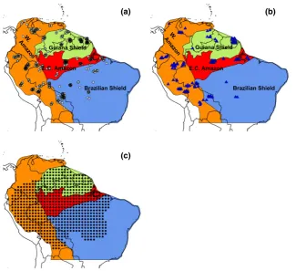
Secondly, we greatly extend the spatial coverage of observations. The first large-scale studies of Amazon forest dynamics (Baker et al., 2004; Malhi et al., 2004; Phillipset al., 2004) focused on the western, and central and eastern portions of the basin, but included few data from forests on the Guiana and Brazilian Shields (Fig. 1). These areas, however, have distinctive soils,
climate, forest structure and species composition (e.g. ter Steegeet al., 2006; Feldpauschet al., 2011). Here, we use data from these regions to test whether the para-digm of a positive association between woody NPP and stem mortality rates, linked to a reduction in AGB, is found across the full range of South American lowland moist tropical forests.
In terms of the analysis of the DGVMs, we aim firstly to establish the reliability of land vegetation simulation for the Amazon basin by comparison of modelling results with kriged maps of field observa-tions of WP, mortality and AGB that illustrate the major patterns of variation in these variables. We then test how well the four DGVMs capture these spatial patterns and the overall magnitude of AGB and WP. Finally, we explore the relationships between simu-lated AGB, WP and sw. By comparing our findings from the analysis of the observations and simulation results, we conclude by making recommendations for model developments and data collection that will improve our ability to model Amazonian vegetation carbon stocks.
(a)
(c)
(b)
[image:4.595.128.454.355.652.2]Materials and methods
Plot observations
We used tree inventory data from permanent sample plots located throughout Amazonia compiled as part of the RAIN-FOR and TEAM networks to estimate stocks (AGB) and fluxes of carbon (woody NPP, stem and biomass mortality) within Amazonian forest stands (Fig. 1). For analysis of AGB, we used the data for the 413 plots analysed by Mitchard et al.
(2014) (Fig. 1a). For properties which can only be calculated by observing change over time and thus require more than one census, plots in intact, moist, lowland (<1000 m asl) forest were chosen which had a minimum total monitoring period of 2 years between 1995 and 2009 inclusive. Data for 167 plots that met these criteria for analysis of dynamic properties were downloaded from ForestPlots.net (Lopez-Gonzalezet al., 2011, 2012; Johnsonet al., 2016; Fig. 1b and Table S1) and the TEAM website (http://www.teamnetwork.org/data/query; data set identifier codes 20130415013221_3991 and 20130405063033_ 1587). For this data set, mean plot size is 1.09 ha, the mean date of the first census is 2000.2 and the mean date of the final census is 2008.5. Mean census interval length is 3.70 years and plot mean total monitoring period is 8.3 years. Most of the plots were monitored for most of the time period: on average, 76% of plots were being monitored in any given year from 2000–2008 (Fig. S1). All trees with a diameter at breast height (dbh) greater than 10 cm were included in the analyses.
Plots were classified into four regions of lowland moist forest defined by the nature and geological age of the soil substrate (Fig. 1; Feldpauschet al., 2011). The soils and forests of the Gui-ana and Brazilian Shields have developed on old, Cretaceous, crystalline substrates, whereas the forests of Western Amazonia are underlain by younger Andean substrates and Miocene deposits (Irion, 1978; Quesadaet al., 2010; Higginset al., 2011). East-central Amazonia contains reworked sediments derived from the other three regions that have undergone almost contin-uous weathering for more than 20 million years, leading to very nutrient poor soils (Irion, 1978; Quesadaet al., 2010). Previous comparative studies have noted substantial differences in forest dynamics between Western and East-central Amazonia (Baker
et al., 2004, 2014; Quesadaet al., 2012), but largely excluded for-ests on the Guiana and Brazilian Shields. This classification therefore allows us to test the impact of including these distinc-tive forests on Amazon-wide patterns of forest dynamics.
Above-ground biomass
For AGB values, we used the data set presented by Mitchard
et al.(2014) and Lopez-Gonzalezet al.(2014). In brief, for this data set, the AGB (Mg DW ha1) of each plot was calculated using the Chave et al. (2005) moist forest allometric equa-tion which includes measurements of diameter, wood density and height:
AGB¼
Pn
1ð0:0509qD2HÞ
1000 ; ð2Þ
where D is stem diameter (cm), q is stem wood density (g cm3),His stem height (m) andnis the number of trees in the stand. We retained the use of this biomass equation for this study, instead of using the recent biomass equation of Chaveet al.(2014), to provide estimates ofWPthat are consis-tent with Mitchardet al. (2014). Estimates of AGB for moist tropical forests are in fact similar using either equation (Chave
et al., 2014). The height of each tree was estimated from tree diameter using a height-diameter Weibull equation with dif-ferent coefficients for each region, based on field-measured, height-diameter relationships (Feldpausch et al., 2011). We used this method to estimate tree height, rather than predict-ing height on the basis of climate as in Chave et al. (2014), because among moist forests in Amazonia, the principal varia-tion in height/diameter allometry is due to the contrast between the particularly tall-statured forests on the Guiana Shield and shorter-statured forest in other regions (Feld-pausch et al., 2011). This difference is related to the unique species composition of forests on the Guiana Shield rather than variation in climate (Feldpauschet al., 2011). The wood density of each tree was assigned on a taxonomic basis from the pan-tropical database of Zanne et al. (2009) and Chave
et al. (2009), following Baker et al. (2004). Mean plot wood density values were used when taxonomic information was missing for individual trees.
To estimate total above-ground woody biomass, we assumed that carbon is 50% of total dry biomass (Penman
et al., 2003) and to account for the unmeasured, small trees (<10 cm), we added an additional 6.2% of carbon to each of the plots, following Malhiet al.(2006). We do not include the unknown contributions from lianas, epiphytes, necromass, shrubs and herbs.
Mortality and productivity
Stem mortality rates were calculated as the exponential mor-tality coefficientl[% yr1; Sheil & May (1996)]:
l¼lnðn0Þ lnðn0ndÞ
t 100; ð3Þ
where n0is the number of stems at the start of the census
interval,ndis the number of stems that die in the interval and
tis the census interval length. As estimates of mortality rates in heterogeneous populations are influenced by the census interval, we standardized our estimates of lto comparable census intervals using the equation of Lewiset al.(2004). We calculated corrected values of lfor each census interval for each plot in the data set, and calculated average values ofl per plot, weighted by the census interval length.
veg-etation models as DGVMs typically partition total above-ground NPP into different carbon pools using various carbon allocation algorithms, ranging from fixed coefficients (e.g. INLAND) to approaches based on resource limitation (e.g. ORCHIDEE). For comparison with measurement data, we used the fraction of simulated above-ground NPP that the models allocate to woody growth. Both the observed measure-ments and models exclude the contribution toWPthat is made by the loss and regrowth of large woody branches. This com-ponent is approximately 1 Mg C ha1a1in Amazonian for-ests or 10% of above-ground NPP (Malhiet al., 2009).WLwas calculated as the sum of the biomass of all trees that died within a given census interval.
Estimates ofWPandWLare influenced by the census inter-val over which they are calculated, because more trees will recruit and die without being recorded during longer census intervals (Talbotet al., 2014). We followed the methods of Tal-botet al.(2014) for calculatingWPwith forest inventory data to correct for this bias (Supporting information, Appendix S1). Thus, we calculatedWPas the sum of (i) the growth of trees that survive the census period, and the estimated growth of (ii) trees that died during the census interval, prior to their death, (iii) trees which recruited within the interval, and (iv) trees that both recruited and died during the census interval. Similarly, to calculateWL,we summed the biomass of trees that die within a census interval with components (ii) and (iv) above. We calculated corrected values ofWPandWLfor each census interval for each plot in the data set, and calculated average values per plot, weighted by census interval length.
Analysis of observational data
The current paradigm for Amazonian forests suggests thatWP andlare positively correlated and that both correlate nega-tively with AGB (Malhiet al., 2002; Quesadaet al., 2012). We tested whether these relationships are supported by the data from across South American tropical lowland moist forest, including plots from the Guiana and Brazilian Shield. Firstly, we explored whether different regions have distinctive patterns of carbon cycling by comparingWP, WL,land AGB among the four regions usingANOVA. Secondly, we explored the relation-ships between these terms using generalized least squares regression. We tested whetherWPand eitherWLorlwere sig-nificantly related to AGB and whether these relationships dif-fered among the four regions. We accounted for spatial autocorrelation by specifying a Gaussian spatial correlation structure, which is consistent with the shape of the semivari-ograms for these forest properties across the plot network (Fig. S2). Stem mortality rates and absolute rates of woody bio-mass loss were log-transformed prior to analysis to ensure the residuals were normally distributed. Model evaluation was performed on the basis of Akaike information criterion (AIC) values. Analyses were carried out using thenlmepackage inR (R Development Core Team, 2012; Pinheiroet al., 2015).
Model simulations and comparison with observations
We tested how well a range of DGVMs perform for Amazo-nia by comparing observed AGB,WPandswto the output
from four DGVMs. The DGVMs included in this study are the joint uk land environment simulator (jules), v. 2.1. (Best
et al., 2011; Clarket al., 2011), the Lund-Potsdam-Jena DGVM for managed Land (LPJmL; Sitch et al., 2003; Gerten et al., 2004; Bondeauet al., 2007), the INtegrated model of LAND surface processes (INLAND) model (a development of the IBIS model, Kuchariket al., 2000) and the Organising Carbon and Hydrology In Dynamic EcosystEms (ORCHIDEE) model (Krinneret al., 2005). A brief description of each of the four models and how output data are derived is included in the supplementary information (Appendix S2). The models each followed the standardized Moore Foundation Andes-Ama-zon Initiative (AAI) modelling protocol (Zhanget al., 2015). The simulated region spanned 88°W to 34°W and 13°N to 25°S. Simulations from each model included a spin-up per-iod from bare ground of up to 500 years with pre-industrial atmospheric CO2 (278 ppm). The models were then forced by recycling 39 year, 1° spatial resolution, bias-corrected NCEP meteorological data (Sheffield et al., 2006) for 1715– 2008 with increasing CO2concentrations, as in Zhang et al. (2015). Figure S3 shows the spatial distribution of mean meteorological variables for 2000–2008 across the Amazon basin. As well as precipitation, temperature and short-wave radiation we also show maximum cumulative water deficit (MWD), calculated from monthly precipitation values to indicate drought severity across the basin, as in Aragaoet al.
(2007). The time period of model output is 2000–2008. To compare simulated woody NPP with observedWP, cor-rections were applied to the simulated total woody NPP to calculate above-ground woody NPP only, by assuming a below-ground to above-ground allocation ratio of 0.21 (Malhi
et al., 2009). In the case of JULES, only a fraction of the NPP is allocated to biomass growth, as the remainder is allocated to ‘spreading’ of vegetated area–an increase in the fraction of grid cell cover (Cox, 2001). To facilitate comparison with observations and other models, we therefore rescaledWPfrom JULES, retaining the relative allocation to wood but assuming that all of the NPP was used for growth.
observed values. The median percentage bias between the leave-one-out cross-validation and the measured plot values was 13.6%, 12.7% and 23.0% for AGB,WPand stem mortality rate respectively.
We do not intend the kriged maps to be a detailed, accurate description of Amazon forest properties: ecological patterns are a mix of smooth gradients (e.g. related to climate) and more abrupt boundaries (e.g. related to edaphic properties) that cannot be shown using these methods. Rather, we intend these maps as broad scale tools to provide a means of evaluat-ing the performance of the vegetation models.
Finally, we compared how well the DGVMs captured the mean and variability in AGB, WPand sw (calculated using average values forWPand AGB across all grid cells for 2000– 2008 from model outputs using Eqn 1) for grid cells where there is observational data, and contrast the controls on AGB between observations and models in terms ofWPand mortal-ity. We acknowledge that the models will predict a small increase inWPover the time period of study due to CO2 fertil-ization (~0.35 Mg C ha1a1; Lewiset al., 2009). However, the effect of this process on estimates ofswis small.
Results
Observed links between woody biomass, mortality and productivity
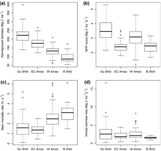
There is a strong variation in AGB (F3,163=72.1, P<0.001), l (F3,163=23.6, P<0.001) and WP (F3,163=22.7,P<0.001) among the four regions, but not WL(F3,163=1.49, ns; Table 1, Fig. 2). Forests on the Gui-ana Shield are characterized by the highest AGB of all Amazonian forests, associated with low stem mortality rates and highWP(Fig. 2a–c). East-central Amazon for-ests also have comparatively high AGB and similar, very low stem mortality rates. However,WPis lower in these sites (Fig. 2b). Compared with these regions, forests in the western Amazon and on the Brazilian Shield have lower AGB. However, the lower biomass in these two
regions is associated with different patterns inWP. In the western Amazon, the lower biomass values are associ-ated with highWP(Fig. 2a–c). In contrast, the particu-larly low biomass forests of the Brazilian Shield have high rates of stem mortality and lowWP(Fig. 2a–c).
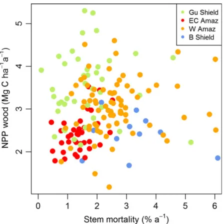
Analysis of the relationships using generalized least squares allows the relative importance of WP and l for determining AGB to be explored in more detail. Stem mortality rate is the key parameter that controls variation in AGB (Table 2, Fig. 4c). This rela-tionship between AGB and stem mortality rates is not because there is a correlation between AGB and stem number, as these two variables are unrelated (Fig. S6). In contrast, the alternative measure of mor-tality, WL, is not related to AGB (Fig. 4b): all models including stem mortality rates, rather than WL, show substantially better fit and lower AIC values (Table 2).
The effect of stem mortality rate on AGB also differs among regions (Fig. 4c). For example, for a stem mortal-ity rate of 1.5% yr1, forests on the Guiana Shield store approximately 75% more carbon as (above-ground) wood than forests on the Brazilian Shield (Fig. 4c). In addition, the strength of the relationship between AGB and stem mortality rates varies among regions: the slope of this relationship is comparatively shallow among the plots in western Amazonia (Fig. 4c). Finally, WP is significantly positively correlated with variation in AGB, although the relationship is weak (Table 2, Fig. 4a).
Model projections and comparison with observations
[image:7.595.78.549.530.701.2]The comparisons of simulated AGB and above-ground WP reveal considerable differences both between the individual models and between the models and obser-vations (Table 3, Figs 5, 6, S7 and S8). For the whole of
Table 1 Observed forest properties (meanSE) calculated from plot data for each region of Amazonia
Basin Guiana Shield
East-central Amazon
Western
Amazon Brazilian Shield
Mean above-ground biomass (Mg C ha1) 153.482.82
n=413
211.915.03
n=110
167.644.95
n=78
126.262.38
n=149
107.734.48
n=76 Mean above-ground woody productivity
(Mg C ha1yr1)
2.970.06
n=167
3.510.13
n=41
2.410.07
n=37
3.060.07
n=76
2.400.15
n=13 Stem-based mortality rate (% yr1) 1.960.08
n=167
1.660.16
n=41
1.380.08
n=37
2.620.12
n=76
3.190.38
n=13 Mean above-ground biomass losses
(Mg C ha1yr1)
2.460.13
n=167
3.060.44
n=41
2.120.16
n=37
2.430.15
n=76
1.570.12
n=13 Mean wood density (g cm3) 0.630.00
n=413
0.690.00
n=110
0.670.01
n=78
0.580.00
n=149
0.610.01
n=76 Basal area (m2ha1) 26.645.53
n=413
29.100.49
n=110
28.240.51
n=78
25.980.41
n=149
22.730.66
the Amazon basin, mean AGB is highest for ORCHI-DEE, and lowest for INLAND; in contrast, woody NPP is highest for LPJmL and lowest for JULES (Table 3). Compared with the plots, different models over- and
underestimate mean AGB (Table 3). However, the model ensemble mean AGB value (163.87 Mg C ha1) is close to the observed mean (153.48 Mg C ha1). In con-trast, all models overestimate above-ground WP
[image:8.595.129.445.56.352.2]Fig. 2 Boxplots of plot measurements of (a) above-ground biomass, (b) above-ground woody productivity, (c) stem mortality rates and (d) absolute rates of woody biomass loss in four regions of Amazonia. Gu Shld=Guiana Shield, EC Amaz=East Central Amazon, W Amaz=Western Amazon, B Shld=Brazilian Shield.
Table 2 Generalized least squares models relating AGB to variation in (A) above-ground woody productivity (WP), stem mortality rates (l) or rates of woody biomass loss (WL); (B)landWP; (C)WLandWPamong 167 plots across four regions of Amazonia. Mod-els incorporated region as an additional factor and interactions as appropriate. Terms for mortality were log-transformed before analysis. All models incorporated a Gaussian spatial error correlation structure to account for spatial autocorrelation. The model with the strongest support is highlighted in bold; this model was used to quantify the relationships in Fig. 3
Model Terms Interactions Log likelihood AIC Pseudorsquared
A. Including either mortality or growth
1 l,Region 813.7 1643.3 0.65
2 WL,Region 830.1 1676.3 0.57
3 WP, Region 829.3 1674.5 0.58
B. IncludingWPandlas mortality term
4 WP,l,Region 810.8 1639.6 0.66
5 WP,l,Region l9Region 805.0 1634.0 0.68
6 WP,l,Region WP9Region 808.8 1641.6 0.67
C. IncludingWPandWLas mortality term
7 WP,WL,Region 829.0 1676.1 0.58
8 WP,WL,Region WL9Region 826.7 1677.4 0.59
9 WP,WL,Region WP9Region 826.6 1677.2 0.59
[image:8.595.47.527.467.625.2]compared with the mean for the plots, by between 36% (JULES) and 234% (LPJmL; Table 3, Fig. 5). Variation in sw inevitably reflects the variation in mean AGB and woody NPP with average values for ORCHIDEE and JULES (27.9 and 33.2 years) approximately twice the values for INLAND and LPJmL (16.7 and 17.5 years).
There are considerable differences between the obser-vations and the predictions across the four models in the spatial variability of AGB andWP(Figs 5, 6 and S7). JULES and INLAND both simulate very little spatial heterogeneity in AGB in the Amazon basin, in contrast to the strong pattern in the observations: compared with the observations, they simulate a very narrow range of AGB values and underestimate both the AGB of the Guiana Shield and the basin as a whole (Table 3, Fig. 5c, e). LPJmL and ORCHIDEE display greater vari-ability in their predictions of AGB (Fig. 5g, i). However, LPJmL predicts highest AGB in the north-west of the basin in contrast to the observations (Fig. 5i). ORCHI-DEE is the only model that provides a reasonable match with the spatial patterns in the observations, but this model still overestimates AGB for most of the basin compared with the plot observations (Table 3, Fig. 5g).
In terms ofWP, LPJmL (Fig. 5j) is the only model that captures the higher observed values in the Guiana Shield and Western Amazon compared with the Brazil-ian Shield and East-central Amazon (Fig. 5b). In con-trast, INLAND, ORCHIDEE and JULES simulate very little variability in WP across the majority of basin (Fig. 5d, f, h).
For all models, the spatial variation inswis similar to that of AGB (Fig. 6). LPJmL demonstrates the greatest spatial variation in residence times with the highest val-ues found in the north-west of the basin (Fig. 6). JULES and INLAND display little variation in swacross the basin. Overall, JULES, LPJmL and INLAND display a much stronger positive relationship between woody NPP and AGB (Fig. 7) than seen in the observations (Fig. 4a), although the form of this relationship varies. In contrast, the relationship predicted by ORCHIDEE matches the variability and form of the relationship
between woody NPP and AGB from the plot data com-paratively well (Fig. 7).
Simulated AGB andWP from all four models show strong relationships with climatological drivers. Corre-lations between WP and precipitation are particularly strong for INLAND and LPJmL and all models apart from JULES exhibit strong correlations between rainfall and AGB (Fig. S9). Weaker correlations are observed between temperature and short-wave radiation and simulatedWPand AGB (Fig. S10).
Discussion
Understanding spatial variation in the AGB of Amazon forests
[image:9.595.70.547.105.180.2]Overall, our results extend and enrich the original para-digm concerning the controls on forest dynamics in Table 3 Basin mean values, standard errors and root mean square error (RMSE) for above-ground wood biomass (AGB; Mg C ha1) and above-ground woody net primary productivity (woody NPP; Mg C ha1yr1) from the plot observations and mean ues from four DGVMs for the plot locations. A below-ground to above-ground allocation ratio of 0.21 is applied to the DGVM val-ues to convert from total NPP wood to above-ground woody NPP
Model
AGB (Obs mean=153.48) WP(Obs mean=2.97)
AGB wood AG NPP wood
ORCHIDEE JULES INLAND LPJmL ORCHIDEE JULES INLAND LPJmL
Model mean 218.003.16 137.932.09 125.431.35 174.102.89 7.800.10 4.050.09 7.460.11 9.920.10
RMSE 91.84 76.98 61.36 73.65 5.00 1.89 4.73 7.06
NPP, net primary productivity; DGVMs, dynamic global vegetation models.
[image:9.595.322.546.435.660.2]Amazonia. The previous paradigm described corre-lated west to east gradients inWP, stem mortality rates and AGB across the Amazon basin, maintained by a soil-mediated, positive feedback mechanism (Malhi et al., 2004; Quesada et al., 2012). Our findings agree that variation in mortality is the key driver of variation in AGB across Amazonian forests (Table 2, Fig. 4). However, our results modify the current paradigm about variation in forest dynamics in Amazonia in four important ways.
Firstly, the plot data demonstrate that there is no cor-relation betweenWP(above-ground woody productiv-ity) and stem mortality rates with the new, broader data set: they vary independently (Fig. 3). Previous studies have strongly focused on western Amazonia and some East-central Amazon sites. However, the inclusion of data from the Guiana Shield in particular demonstrates that low stem mortality rates can also be associated with highWP(Fig. 3).
Secondly, our results demonstrate that variation in stem mortality rates, rather than absolute rates of car-bon loss, is the key aspect of mortality that determines variation in AGB. The lack of correlation between AGB and absolute rates of biomass loss (Fig. 4b) is somewhat surprising: for a forest stand at approximately steady state, we might expect this relationship to at least mir-ror the weak correlation between AGB and standWP (Fig. 4a). This result may be because estimates of abso-lute AGB loss are subject to greater sampling error than WPdue to stochastic variation in tree mortality (e.g. see wide variation in values on thexaxis of Fig. 4b). Sam-pling over longer time intervals may reveal stronger correlations between absolute rates of biomass loss and AGB.
In contrast to these patterns for absolute rates of loss of biomass, there are strong relationships between stem mortality rates and AGB (Fig. 4c). This result suggests that variation in the numbers and diameters of trees that die in different locations is a key control on AGB: high rates of stand-level biomass loss and WP can be associated with high AGB if stem mortality rates are low, and biomass loss is concentrated in a few large trees, but can also be associated with comparatively low AGB if stem mortality rates are high, and mortality is concentrated in a larger number of smaller trees (Fig. 4). Stem mortality rates may influence AGB because they affect the size structure of forests: demo-graphic theory demonstrates how higher stem mortal-ity rates are associated with a steeper slope of tree size/ frequency distributions and therefore fewer large trees (Coomes et al., 2003; Muller-Landau et al., 2006). In turn, variation in the number of large trees is a key pre-dictor of spatial variation in biomass among forest plots (e.g. Baker et al., 2004; Baraloto et al., 2011). Impor-tantly, this result indicates that incorporating stem diameter distributions within modelling frameworks will be important for obtaining accurate predictions of AGB.
Thirdly, our results resolve a paradox in the original paradigm–thatWPshowed a negative correlation with AGB (Malhi, 2012). Here, with a broader range of sites, the expected positive correlation is found, although the strength of the relationship remains weak (Fig. 4a). Pos-itive correlations between AGB andWPare a feature of the output of DGVMs (e.g. Fig. 7). This analysis, at least to an extent, demonstrates consistency between one aspect of the models and the data, although the
[image:10.595.53.524.471.662.2]strength of the observed relationship is much weaker than that specified by the models (Figs 4a and 7).
Fourthly, the vertical offsets of the relationships between stem mortality rates and AGB among regions suggest that variation in the identity and height/di-ameter allometry of trees in different parts of Amazo-nia is also important for understanding variation in AGB. For example, observations from plots on the Guiana Shield show that these forests have very high AGB values for a given stem mortality rate (Fig. 4c), associated with surprisingly high WP (Fig. 4a). This result implies that AGB is concentrated within trees with greater heights and/or higher wood density in these forests compared with other regions. A combi-nation of good soil structural properties that promotes low stem mortality rates, and relatively high soil phosphorus concentrations that promote high produc-tivity (Quesada et al., 2012) could conceivably allow these forests to attain the combination of high basal area, tree heights and wood density that results in particularly high AGB. Comparatively high levels of soil fertility are possible as this region may receive significant additions of inorganic phosphorus and other mineral nutrients from dust deposits; this region of the Amazon is believed to receive the highest amounts of dust from Saharan Africa (Mahowald et al., 1999, 2005). Alternatively, the greater heights, wood density and WP of these forests may be related to their distinctive taxonomic composition; these for-ests contain a high proportion of stems of large-sta-tured species of Leguminosae (ter Steege et al., 2006). These species may achieve greater phosphorus-use efficiency during photosynthesis or allocate a greater proportion of NPP to woody growth – both are pro-cesses that lead to higher AGB forests (Malhi, 2012). Variation in species composition, or biogeography, related to historical patterns of species dispersal over long timescales is known to be a factor in determining the high AGB and WP of forests in Borneo compared with Amazonia (Banin et al., 2014). Similar processes may also be important within Amazon forests.
Conversely, forests on the Brazilian Shield towards the southern margins of Amazonian forests have par-ticularly low AGB for a given stem mortality rate, associated with generally low values forWP and high values of l (Marimon et al., 2014; Fig. 4). Such low woody productivity, high stem mortality rates and potentially low stature forest in these locations are likely to be caused by repeated moisture stress and/ or fire (Phillips et al., 2009; Brando et al., 2014): towards the southern margins of Amazonia, AGB approximately halves with a doubling in moisture stress quantified using the maximum climatological water deficit (Malhiet al., 2015).
Overall, our findings emphasize the pre-eminent role of variation in stem mortality rates for controlling AGB, but indicate that variation in woody NPP is also impor-tant. They also emphasize how the links between AGB, tree growth and mortality are modified by species com-position and the allocation of carbon to dense or light wood, or growth in height (Fig. 4c). Clearly, more com-prehensive analyses of these sites including environ-mental data (cf Quesada et al., 2012) are required to tease apart the underlying drivers of these patterns. Additional data from low AGB forests in stressful envi-ronments across Amazonia, such as on white sand or peat (Baraloto et al., 2011; Draper et al., 2014), would also be valuable. Such low AGB forests have typically been excluded from ecosystem monitoring but may prove particularly informative to constrain the form of the relationships betweenWP, stem mortality rates and AGB.
Finally, our results suggest that the sensitivity of AGB to variation in stem mortality rates is greater in high AGB forests which have the lowest stem mortality rates (Fig. 4c). Increasing mortality rates are a feature of many threats faced by tropical forests, whether dri-ven by increased growth, drought or fire, and extrapo-lations from forest plot data have been used to argue that such increases may substantially reduce the carbon stocks and carbon sink potential of these ecosystems (e.g. Lewis, 2006; Brienenet al., 2015). Our results indi-cate that forests with the highest AGB values will be most sensitive to a given increase in stem mortality rates (Fig. 4c). In addition, our results suggest that there may be regional differences in the sensitivity of the carbon stocks of Amazonian forests to changing stem mortality rates. For example, increases in stem mortality rates in the Guianas will not lead these forests to become structurally identical to western Amazon for-ests; they will follow their own trajectory related to their distinctive composition (Fig. 4c).
Understanding spatial patterns in model simulations
Simulated AGB in the four DVGMs depends on the bal-ance of woody NPP and losses due to the turnover of woody tissue, ‘background’ mortality, specific pro-cesses such as drought, or more generic ‘disturbance’ (Table 4). Here, we consider how these models simu-late woody NPP and mortality to understand simusimu-lated patterns of AGB.
constant in JULES (Table 4) and simulatedswis largely invariant (Figs 5 and 6). As a result, there is a positive relationship between simulated AGB and NPP for this model (Fig. 7). However, interestingly, the relationship between AGB and NPP in JULES is nonlinear and sug-gests that there is an upper limit to the amount of AGB that can be simulated in JULES. This arises from the particular allocation scheme used in JULES where NPP is partitioned into biomass growth of existing vegeta-tion or into ‘spreading’ of vegetated area (Cox, 2001). This partitioning into growth/spreading is regulated by LAI so that as LAI increases, less NPP is allocated to biomass growth. In this formulation, a maximum LAI value is prescribed which effectively sets a cap on bio-mass growth in the model, as at this point all of the NPP is directed into ‘spreading’ and none of it into growth of the existing vegetation. When a PFT occupies all of the available space in a grid cell and therefore cannot expand in area, all of the NPP effectively enters the litter via an assumed ‘self-shading’ effect (Table 4; Huntingfordet al., 2000).
INLAND simulates slightly more variation in WP across the basin than JULES. However, most of this variation is observed at the basin fringes, which may be explained by INLAND’s nonlinear relationship betweenWPand rainfall; where annual rainfall exceeds 2 m yr1, simulatedWPdoes not vary with changes in
precipitation (Fig. S9). As a result, there is a very strong relationship between AGB and NPP (Fig. 7), and AGB varies little across Amazonia, similar to JULES (Fig. 5).
Productivity in LPJmL is much more strongly related to rainfall and MWD than either JULES or INLAND (Fig. S9), which is consistent with previous studies that have shown LPJ to be more sensitive to soil moisture stress than other models such as MOSES-TRIFFID, the precursor model to JULES (Galbraithet al., 2010). As a result, we observe more spatial variation across the basin in WP. More generally, mortality is also more complex in this model and is a function of negative growth, heat stress and bioclimatic limits and includes disturbance from fire (Table 4; Sitch et al., 2003). As result, in contrast to the other models, there are correla-tions betweensw, rainfall and MWD in LPJmL (Fig. S9) resulting in substantial spatial variation in AGB and the highest AGB values in the wet, north-west of the basin.
ORCHIDEE also demonstrates spatial variation in WP which is nonlinearly correlated with rainfall (Fig. S9). Carbon residence times and AGB in ORCHI-DEE are similarly, but more strongly, correlated with rainfall and MWD thanWP, and as a result, there is a greater variability in the relationship between AGB and NPP for this model (Fig. 7) and greater spatial variation in AGB (Fig. 5).
How can we improve simulations of spatial variation in DGVMs based on the observations?
A possible explanation for some of the disparities between the observations and model simulations may be the differences in how disturbance influences both data-sets: the forest plots will experience the full range of dis-turbances that occur in natural forest, whilst the simulations are limited to reflecting only the effect of modelled processes. However, in broad terms, the degree and intensities of disturbance are likely to be comparable: amongst the DVGMs in this study, mortality is modelled based on a wide range of relevant processes –a back-ground rate due to tree senescence, competition for light, drought and externally forced disturbance (Table 4). Rare but intense, large-scale disturbances related to blow-downs are excluded from the simulations and such dis-turbances can have landscape-scale effects (Chambers et al., 2013), but their extreme rarity and patchiness at a regional scale makes it unlikely that they substantially alter or determine broad scale patterns of forest structure and dynamics (Espı´rito-Santoet al., 2014).
[image:12.595.49.274.104.349.2]A key finding from the observational data is that variation in stem mortality rates determines spatial variation in AGB (Fig. 3). This finding implies that mor-tality must be modelled on the basis of individual Table 4 Comparison of woody biomass mortality/turnover
schemes used by the four DGVMs of this study. Where speci-fic values are provided, these relate to the dominant PFT assumed by the models over our area of study
INLAND JULES LPJmL ORCHIDEE
1. Turnover of woody tissue Fixed/
variable
Fixed Fixed Variable Fixed
Woody turnover time (sw)
25 years 200 years 30 years
2. Background disturbance rate
Yes/No? Yes Yes No No
% a1 0.05 0.05
3. Specific drivers of mortality Negative
carbon balance
No No Yes No
Fire Yes No Yes No
Drought No No Yes No
Competition for light
No Yes Yes No
References Kucharik et al. (2000) Clark et al. (2011) Sitch et al. (2003) Delbart et al. (2010)
(a) (b)
(c) (d)
(e) (f)
(g) (h)
(i) (j)
[image:13.595.78.526.52.658.2]stems, and suggests stem-size distributions are impor-tant for predicting variation in AGB. However, the architecture of the DVGMs in this study does not incor-porate stem-size distributions, or individual-based mortality rates. In contrast, three of the four models in
this study employ a fixed value of sw(a PFT-specific woody turnover rate, Table 4), to model a background rate of woody biomass loss, related to growth. In the models where these constant terms dominate mortality (e.g. JULES/INLAND), inevitably, the patterns of AGB (a) (b)
(c) (d)
(e) (f)
[image:14.595.51.521.64.590.2]mirror those ofWPand do not match the observations. Even in ORCHIDEE which simulates the highest bio-mass in the north-east of the basin similar to the obser-vations (Fig. 5), this apparent correspondence between the model and observations is not because this model effectively models tree mortality: like JULES and INLAND, ORCHIDEE also employs a constant mortal-ity rate (Table 4; Delbart et al., 2010). In addition, the finding that variation in stem mortality determines variation in AGB implies that introducing simple rela-tionships between mortality andWP, such as linkingsw to NPP (Delbart et al., 2010) will not improve predic-tions for the whole basin. For example, the forests of the Guiana Shield, where forests have high WP and high AGB but low stem mortality rates, will not be accurately modelled using the technique employed by Delbartet al.(2010).
A second key reason for discrepancies between the observations and models is that the key processes driv-ing variation in the observations differ from the mod-elled processes. For example, when mortality is included as a dynamic process in the DGVMs, such as in LPJmL, mortality strongly reflects the variability in that process: moisture stress across the basin in the
context of LPJmL. In contrast, stem mortality rates in Amazonian plots ultimately strongly respond also to edaphic properties such as soil physical properties (Quesadaet al., 2012).
These findings suggest several ways in which veg-etation models could be developed. Firstly, mortality needs to be effectively incorporated in these models, preferably through incorporating stem mortality rates (l), rather than average carbon residence times (sw), as a means of modelling the loss of woody carbon. The process of stem mortality is much more amenable for linking with the ultimate drivers of tree death, such as hydraulic failure, and is the key driver of variation in the size structure and AGB of Amazonian forests. We note that there have been positive advances in modelling mortality processes more mechanistically in DGVMs (e.g. Fisher et al., 2010, 2015) and that there is a considerable focus at present in improving the representation of vegeta-tion dynamics in DGVMs (e.g. Verbeeck et al., 2011; De Weirdt et al., 2012; Castanho et al., 2013; Haverd et al., 2014; Weng et al., 2015). Secondly, DGVMs need to focus on including more functional diversity and variation in height/diameter relationships to
[image:15.595.149.464.57.381.2]capture regional differences in the carbon dynamics of Amazon forests. Thirdly, mortality processes need to be linked to edaphic properties such as a mea-sure of soil structure/stability, and WP to spatially varying soil nutrients to ensure that not only climate stress influences the spatial variation of AGB that is predicted by DGVMs. Finally, our study highlights the importance of size structure in shaping forest dynamics. To model tropical forest dynamics effec-tively, ‘average individual’ approaches which do not account for size distributions in tropical forests are insufficient. Several different aspects of these recom-mendations are already being implemented in emerging model frameworks (e.g. Fyllas et al., 2014; Sakschewski et al., 2015) and we look forward to testing the predictions of the next generation of veg-etation models against baseline datasets of forest structure and dynamics.
Acknowledgements
This paper is a product of the European Union’s Seventh Frame-work Programme AMAZALERT project (282664). The field data used in this study have been generated by the RAINFOR net-work, which has been supported by a Gordon and Betty Moore Foundation grant, the European Union’s Seventh Framework Programme projects 283080, ‘GEOCARBON’; and 282664, ‘AMAZALERT’; ERC grant ‘Tropical Forests in the Changing Earth System’), and Natural Environment Research Council (NERC) Urgency, Consortium and Standard Grants ‘AMAZO-NICA’ (NE/F005806/1), ‘TROBIT’ (NE/D005590/1) and ‘Niche Evolution of South American Trees’ (NE/I028122/1). Additional data were included from the Tropical Ecology Assessment and Monitoring (TEAM) Network–a collaboration between Conser-vation International, the Missouri Botanical Garden, the Smith-sonian Institution and the Wildlife Conservation Society, and partly funded by these institutions, the Gordon and Betty Moore Foundation, and other donors. Fieldwork was also partially sup-ported by Conselho Nacional de Desenvolvimento Cientı´fico e Tecnolo´gico of Brazil (CNPq), project Programa de Pesquisas Ecolo´gicas de Longa Duracßa˜o (PELD-403725/2012-7). A.R. acknowledges funding from the Helmholtz Alliance ‘Remote Sensing and Earth System Dynamics’; L.P., M.P.C. E.A. and M.T. are partially funded by the EU FP7 project ‘ROBIN’ (283093), with co-funding for E.A. from the Dutch Ministry of Economic Affairs (KB-14-003-030); B.C. [was supported in part by the US DOE (BER) NGEE-Tropics project (subcontract to LANL). O.L.P. is supported by an ERC Advanced Grant and is a Royal Society-Wolfson Research Merit Award holder. P.M. acknowledges support from ARC grant FT110100457 and NERC grants NE/J011002/1, and T.R.B. acknowledges support from a Leverhulme Trust Research Fellowship.
References
Aragao LEO, Malhi Y, Roman-Cuesta RM, Saatchi S, Anderson LO, Shimabukuro YE (2007) Spatial patterns and fire response of recent Amazonian droughts. Geophysi-cal Research Letters,34, LO7701.
Baker TR, Phillips OL, Malhi Yet al.(2004) Variation in wood density determi-nes spatial patterns in Amazonian forest biomass.Global Change Biology, 10, 545–562.
Baker TR, Pennington RT, Magallon Set al.(2014) Fast demographic traits promote high diversification rates of Amazonian trees.Ecology Letters,17, 527–536. Banin L, Lewis SL, Lopez-Gonzalez Get al.(2014) Tropical forest wood production: a
cross-continental comparison.Journal of Ecology,102, 1025–1037.
Baraloto C, Rabaud S, Molto Qet al.(2011) Disentangling stand and environmental correlates of aboveground biomass in Amazonian forests.Global Change Biology,
17, 2677–2688.
Best M, Pryor M, Clark Det al.(2011) The Joint UK Land Environment Simulator (JULES), model description–Part 1: energy and water fluxes.Geoscientific Model Development,4, 677–699.
Bondeau A, Smith PC, Zaehle Set al.(2007) Modelling the role of agriculture for the 20th century global terrestrial carbon balance.Global Change Biology,13, 679–706. Brando PM, Balch JK, Nepstad DCet al.(2014) Abrupt increases in Amazonian tree
mortality due to drought–fire interactions.Proceedings of the National Academy of Sciences of the United States of America,111, 6347–6352.
Brienen R, Phillips O, Feldpausch Tet al.(2015) Long-term decline of the Amazon carbon sink.Nature,519, 344–348.
Castanho A, Coe M, Costa M, Malhi Y, Galbraith D, Quesada C (2013) Improving simulated Amazon forest biomass and productivity by including spatial variation in biophysical parameters.Biogeosciences,10, 2255–2272.
Chambers JQ, Negron-Juarez RI, Marra DMet al. (2013) The steady-state mosaic of disturbance and succession across an old-growth Central Amazon forest landscape.Proceedings of the National Academy of Sciences of the United States of America,110, 3949–3954.
Chave J, Andalo C, Brown Set al.(2005) Tree allometry and improved estimation of carbon stocks and balance in tropical forests.Oecologia,145, 87–99.
Chave J, Coomes D, Jansen S, Lewis SL, Swenson NG, Zanne AE (2009) Towards a worldwide wood economics spectrum.Ecology Letters,12, 351–366.
Chave J, Re´jou-Me´chain M, Bu´rquez Aet al.(2014) Improved allometric models to estimate the aboveground biomass of tropical trees.Global Change Biology,20, 3177–3190.
Clark D, Mercado L, Sitch Set al.(2011) The Joint UK Land Environment Simulator (JULES), model description–Part 2: carbon fluxes and vegetation dynamics. Geo-scientific Model Development,4, 701–722.
Coomes DA, Duncan RP, Allen RB, Truscott J (2003) Disturbances prevent stem size-density distributions in natural forests from following scaling relationships. Ecol-ogy Letters,6, 980–989.
da Costa ACL, Galbraith D, Almeida Set al.(2010) Effect of 7 yr of experimental drought on vegetation dynamics and biomass storage of an eastern Amazonian rainforest.New Phytologist,187, 579–591.
Cox PM (2001) Description of the TRIFFID dynamic global vegetation model. Techni-cal Note 24, Hadley Centre, UK, MeteorologiTechni-cal Office, Bracknell, UK.
Cox PM, Betts R, Collins M, Harris P, Huntingford C, Jones C (2004) Amazonian for-est dieback under climate-carbon cycle projections for the 21st century.Theoretical and Applied Climatology,78, 137–156.
De Weirdt M, Verbeeck H, Maignan Fet al.(2012) Seasonal leaf dynamics for tropical evergreen forests in a process-based global ecosystem model.Geoscientific Model Development,5, 1091–1108.
Delbart N, Ciais P, Chave J, Viovy N, Malhi Y, Le Toan T (2010) Mortality as a key driver of the spatial distribution of aboveground biomass in Amazonian forest: results from a dynamics vegetation model.Biogeosciences,7, 3017–3039. Draper FC, Roucoux KH, Lawson ITet al.(2014) The distribution and amount of
car-bon in the largest peatland complex in Amazonia.Environmental Research Letters,9, 124017.
Espı´rito-Santo FD, Gloor M, Keller Met al.(2014) Size and frequency of natural forest dis-turbances and the Amazon forest carbon balance.Nature Communications,5, 3434. Eva HD, Huber O, Achard Fet al.(2005) A proposal for defining the geographical
boundaries of Amazonia. In:Synthesis of the results from an Expert Consultation Workshop organized by the European Commission in collaboration with the Amazon Cooperation Treaty Organization - JRC Ispra(eds. H.D. Eva and O. Huber), pp. 1–38. Luxembourg Office for Official Publications of the European Communities, Lux-embourg.
Feldpausch TR, Banin L, Phillips OLet al.(2011) Height-diameter allometry of tropi-cal forest trees.Biogeosciences,8, 1081–1106.
Fisher RA, Muszala S, Verteinstein Met al.(2015) Taking off the training wheels: the properties of a dynamic vegetation model without climate envelopes, CLM4.5 (ED).Geoscientific Model Development,8, 3593–3619.
Fyllas N, Gloor E, Mercado Let al.(2014) Analysing Amazonian forest productivity using a new individual and trait-based model (TFS v. 1).Geoscientific Model Devel-opment,7, 1251–1269.
Galbraith D, Levy PE, Sitch S, Huntingford C, Cox P, Williams M, Meir P (2010) Multi-ple mechanisms of Amazonian forest biomass losses in three dynamic global vege-tation models under climate change.New Phytologist,187, 647–665.
Galbraith D, Malhi Y, Affum-Baffoe Ket al.(2013) Residence times of woody biomass in tropical forests.Plant Ecology & Diversity,6, 139–157.
Gatti L, Gloor M, Miller Jet al.(2014) Drought sensitivity of Amazonian carbon bal-ance revealed by atmospheric measurements.Nature,506, 76–80.
Gerten D, Schaphoff S, Haberlandt U, Lucht W, Sitch S (2004) Terrestrial vegetation and water balance– hydrological evaluation of a dynamic global vegetation model.Journal of Hydrology,286, 249–270.
Haverd V, Smith B, Nieradzik LP, Briggs PR (2014) A stand-alone tree demography and landscape structure module for Earth system models: integration with inven-tory data from temperate and boreal forests.Biogeosciences,11, 4039–4055. Higgins MA, Ruokolainen K, Tuomisto Het al.(2011) Geological control of floristic
composition in Amazonian forests.Journal of Biogeography,38, 2136–2149. Huntingford C, Cox P, Lenton T (2000) Contrasting responses of a simple terrestrial
ecosystem model to global change.Ecological Modelling,134, 41–58.
Huntingford C, Zelazowski P, Galbraith Det al.(2013) Simulated resilience of tropical rainforests to CO2-induced climate change.Nature Geoscience,6, 268–273. Irion G (1978) Soil infertility in the Amazonian rain forest.Naturwissenschaften,65,
515–519.
Johnson MO, Galbraith D, Gloor Eet al.(2016) Plot data from: “Variation in stem mortality rates determines patterns of aboveground biomass in Amazonian for-ests: implications for dynamic global vegetation models”. ForestPlotsNET, doi:10.5521/FORESTPLOTS.NET/2016_2.
Krinner G, Viovy N, De Noblet-Ducoudre´ Net al.(2005) A dynamic global vegetation model for studies of the coupled atmosphere-biosphere system.Global Biogeochemi-cal Cycles,19, GB1015.
Kucharik CJ, Foley JA, Delire Cet al.(2000) Testing the performance of a dynamic global ecosystem model: water balance, carbon balance, and vegetation structure.
Global Biogeochemical Cycles,14, 795–825.
Lewis SL (2006) Tropical forests and the changing earth system.Transactions of the Royal Society of London (Series B),361, 195–210.
Lewis SL, Lloyd J, Sitch S, Mitchard ET, Laurance WF (2009) Changing ecology of tro-pical forests: evidence and drivers.Annual Review of Ecology, Evolution, and Sys-tematics,40, 529–549.
Lewis SL, Phillips OL, Sheil Det al.(2004) Tropical forest tree mortality, recruitment and turnover rates: calculation, interpretation and comparison when census inter-vals vary.Journal of Ecology,92, 929–944.
Lopez-Gonzalez G, Lewis SL, Burkitt M, Phillips OL (2011) ForestPlotsnet: a new web application and research tool to manage and analyse tropical forest plot data. Jour-nal of Vegetation Science,22, 610–613.
Lopez-Gonzalez G, Lewis SL, Burkitt M, Baker TR, Phillips OL (2012) ForestPlots.net. Available at: www.forestplots.net (accessed 01 September 2013).
Lopez-Gonzalez G, Mitchard ETA, Feldpausch TRet al.(2014) Amazon forest bio-mass measured in inventory plots Plot Data from “Markedly divergent estimates of Amazon forest carbon density from ground plots and satellites”. ForestPlots-NET, doi:105521/FORESTPLOTSNET/2014_1.
Mahowald N, Kohfeld K, Hansson Met al.(1999) Dust sources and deposition during the last glacial maximum and current climate: a comparison of model results with paleodata from ice cores and marine sediments.Journal of Geophysical Research: Atmospheres (1984–2012),104, 15895–15916.
Mahowald NM, Artaxo P, Baker AR, Jickells TD, Okin GS, Randerson JT, Townsend AR (2005) Impacts of biomass burning emissions and land use change on Amazo-nian atmospheric phosphorus cycling and deposition.Global Biogeochemical Cycles,
19, GB4030.
Malhi Y (2012) The productivity, metabolism and carbon cycle of tropical forest vege-tation.Journal of Ecology,100, 65–75.
Malhi YM, Meir P, Brown S (2002) Forest, carbon and global climate.Philosophical Transactions of the Royal Society (Series B),360, 1567–1591.
Malhi Y, Baker TR, Phillips OLet al.(2004) The above-ground coarse wood produc-tivity of 104 Neotropical forest plots.Global Change Biology,10, 563–591. Malhi Y, Wood D, Baker TRet al.(2006) The regional variation of above-ground live
biomass in old-growth Amazonian forests.Global Change Biology,12, 1107–1138.
Malhi Y, Aragao LEO, Metcalfe DBet al.(2009) Comprehensive assessment of carbon productivity, allocation and storage in three Amazonian forests.Global Change Biol-ogy,15, 1255–1274.
Malhi Y, Doughty CE, Goldsmith GRet al.(2015) The linkages between photosynthe-sis, productivity, growth and biomass in lowland Amazonian forests. Global Change Biology,21, 2283–2295.
Marimon BS, Marimon-Junior BH, Feldpausch TRet al.(2014) Disequilibrium and hyperdynamic tree turnover at the forest–cerrado transition zone in southern Amazonia.Plant Ecology & Diversity,7, 281–292.
Marthews T, Quesada C, Galbraith D, Malhi Y, Mullins C, Hodnett M, Dharssi I (2014) High-resolution hydraulic parameter maps for surface soils in tropical South America.Geoscientific Model Development,7, 711–723.
Meir P, Wood TE, Galbraith DR, Brando PM, da Costa ACL, Rowland L, Ferreira LV (2015) Threshold responses to soil moisture deficit by trees and soil in tropical rain forests: insights from field experiments.BioScience,65, 882–892.
Mitchard ET, Feldpausch TR, Brienen RJet al.(2014) Markedly divergent estimates of Amazon forest carbon density from ground plots and satellites.Global Ecology and Biogeography,23, 935–946.
Muller-Landau HC, Condit RS, Chave Jet al.(2006) Testing metabolic ecology theory for allometric scaling of tree size, growth and mortality in tropical forests.Ecology Letters,9, 575–588.
Negro´n-Jua´rez RI, Koven CD, Riley WJet al.(2015) Observed allocations of pro-ductivity and biomass, and turnover times in tropical forests are not accu-rately represented in CMIP5 Earth system models. Environmental Research Letters,10, 064017.
Nepstad DC, Marisa Tohver I, Ray D, Moutinho P, Cardinot G (2007) Mortality of large trees and lianas following experimental drought in an Amazon forest. Ecol-ogy,88, 2259–2269.
Pan Y, Birdsey RA, Fang Jet al.(2011) A large and persistent carbon sink in the world’s forests.Science,333, 988–993.
Pebesma EJ (2004) Multivariable geostatistics in S: thegstatpackage.Computers & Geo-sciences,30, 683–691.
Penman J, Gytarsky M, Hiraishi Tet al.(2003)Good Practice Guidance for Land Use, Land-Use Change and Forestry. Institute for Global Environmental Strategies, Kami Yamaguchi, Japan.
Phillips OL, Baker TR, Arroyo Let al.(2004) Pattern and process in Amazon tree turn-over, 1976-2001.Philosophical Transactions of the Royal Society of London Series B-Bio-logical Sciences,359, 381–407.
Phillips OL, Araga˜o L, Fisher JBet al.(2009) Drought sensitivity of the Amazon rain-forests.Science,323, 1344–1347.
Pinheiro J, Bates D, DebRoy S, Sarkar D, R Core Team (2016)nlme: Linear and Nonlin-ear Mixed Effects Models. R package version 3.1-127, Available at: http://CRAN.R-project.org/package=nlme, (accessed 03 January 2016).
Quesada C, Lloyd J, Schwarz Met al.(2010) Variations in chemical and physical properties of Amazon forest soils in relation to their genesis.Biogeosciences,7, 1515–1541.
Quesada CA, Phillips OL, Schwarz Met al.(2012) Basin-wide variations in Amazon forest structure and function are mediated by both soils and climate.Biogeosciences,
9, 2203–2246.
Rammig A, Jupp T, Thonicke Ket al.(2010) Estimating the risk of Amazonian forest dieback.New Phytologist,187, 694–706.
R Development Core Team (2012)R: A Language and Environment for Statistical Com-puting. R Foundation for Statistical Computing, Vienna.
Restrepo-Coupe N, da Rocha HR, Hutyra LRet al.(2013) What drives the seasonality of photosynthesis across the Amazon basin? A cross-site analysis of eddy flux tower measurements from the Brasil flux network.Agricultural and Forest Meteorol-ogy,182–183, 128–144.
Rowland L, Da Costa A, Galbraith DRet al.(2015) Death from drought in tropical for-ests is triggered by hydraulics not carbon starvation.Nature,528, 119–122. Sakschewski B, Von Bloh W, Boit Aet al.(2015) Leaf and stem economics spectra
drive functional diversity in a dynamic global vegetation model.Global Change Biology,21, 2711–2725.
Sheffield J, Goteti G, Wood EF (2006) Development of a 50-year high-resolution global dataset of meteorological forcings for land surface modeling.Journal of Climate,19, 3088–3111.
Sheil D, May RM (1996) Mortality and recruitment rate evaluations in heterogeneous tropical forests.Journal of Ecology,84, 91–100.
ter Steege H, Pitman N, Phillips OLet al.(2006) Continental scale patterns of canopy tree composition and function across Amazonia.Nature,443, 444–447.
Talbot J, Lewis SL, Lopez-Gonzalez Get al.(2014) Methods to estimate aboveground wood productivity from long-term forest inventory plots.Forest Ecology and Man-agement,320, 30–38.
Verbeeck H, Peylin P, Bacour C, Bonal D, Steppe K, Ciais P (2011) Seasonal pat-terns of CO2 fluxes in Amazon forests: fusion of eddy covariance data and the ORCHIDEE model. Journal of Geophysical Research Biogeosciences (2005–
2012),116, G02018.
Wang X, Piao S, Ciais Pet al.(2014) A two-fold increase of carbon cycle sensitivity to tropical temperature variations.Nature,506, 212–215.
Weng ES, Malyshev S, Lichstein JWet al. (2015) Scaling from individual trees to forests in an Earth system modeling framework using a mathemati-cally tractable model of height-structured competition.Biogeosciences,12, 2655–
2694.
Zanne AE, Lopez-Gonzalez G, Coomes DAet al.(2009) Global wood density data-base. Dryad Identifier: http://hdlhandle net/10255/dryad, 235.
Zhang K, Almeida Castanho AD, Galbraith DRet al.(2015) The fate of Amazonian ecosystems over the coming century arising from changes in climate, atmospheric CO2, and land use.Global Change Biology,21, 2569–2587.
Zhao M, Running SW (2010) Drought-induced reduction in global terrestrial net pri-mary production from 2000 through.Science,329, 940–943.
Supporting Information
Additional Supporting Information may be found in the online version of this article:
Appendix S1: Calculating above ground woody productiv-ity (WP) from inventory data following Talbotet al.(2014).