A B S T R A C T
We model the combined effects of photoionization and momentum-driven winds from O-stars on molecular clouds spanning a parameter space of initial conditions. The dynamical effects of the winds are very modest. However, in the lower mass clouds, they influence the morphologies
of the HIIregions by creating 10-pc-scale central cavities. The inhomogeneous structures of
the model giant molecular clouds (GMCs) make them highly permeable to photons, ionized gas and supernova ejecta, and the leaking of ionized gas in particular strongly affects their evolution, reducing the effectiveness of feedback. Nevertheless, feedback is able to expel large fractions of the mass of the lower escape velocity clouds. Its impact on star formation is more modest, decreasing final star formation efficiencies by 10–20 per cent, and the rate of change of the star formation efficiency per freefall time by about one third. However, the clouds still form stars substantially faster than observed GMCs.
Key words: stars: formation – ISM: bubbles – HIIregions.
1 I N T R O D U C T I O N
Stellar feedback operates at every scale in the star formation pro-cess and is a crucial ingredient in models of galaxy formation and evolution. Radiation pressure, jets and outflows in the 100 au–1 pc regime may help to set stellar masses and may drive small-scale turbulence (e.g. Li & Nakamura2006; Cunningham et al.2011). Radiative heating by protostars, including the low-mass objects, is also important at these scales for its influence on the fragmenta-tion of the gas (e.g. Krumholz, Klein & McKee2007a; Bate2009; Krumholz et al.2010; Urban, Martel & Evans2010). At intermedi-ate scales, HIIregions (HIIRs), winds and radiation pressure driven
primarily by massive stars profoundly alter the structures and ve-locity fields of giant molecular clouds (GMCs), creating bubbles and champagne flows (e.g. Tenorio-Tagle1979; Whitworth1979), expelling gas from clouds’ potential wells (e.g. Matzner2002) and, in some locations, triggering star formation (e.g. Gritschneder et al.
2009; Walch et al.2011). At galactic scales, the photons, momen-tum and energy produced by these processes and by supernovae (SN) shape the structures of galaxies and the interstellar medium (ISM) and play a major role in globally regulating star formation (e.g. Agertz et al.2013; Hopkins et al.2013).
All star formation occurs in GMCs, so all stellar feedback mecha-nisms interact initially with the host GMC of their originating stars.
E-mail:[email protected]
While SN are likely to be the most important form of feedback on galactic scales, their effects will be modulated by the environment in which they explode. This in turn is modified by the other types of feedback in the interval between the onset of star formation and the demise of the first O-stars. Disentangling the effects of the vari-ous types of stellar feedback is exceedingly difficult from either an observational or theoretical point of view. There has, however, been considerable progress, particularly on the 1–100 pc scales where the dominant mechanisms are photoionization, radiation pressure and stellar winds.
Several authors have examined the issue of the relative or com-bined effects of winds and photoionization. McKee, van Buren & Lazareff (1984) and McCray & Kafatos (1987) argue that wind bub-bles are likely to be trapped by the HIIRs of their driving stars or that the inhomogeneous density fields in clouds are likely to cause the winds to cool on their expansion time-scales or shorter, decreasing their effectiveness. Capriotti & Kozminski (2001) concluded that, except in very dense (>105cm−3) gas, the effects of
photoioniza-tion will dominate. Analytic work by Matzner (2002) also found that wind bubbles were likely to be confined by HIIRs except in the case of very luminous clusters/associations.
Most numerical work has focused on single feedback mecha-nisms and the most popular choice has been HIIRs (e.g. Dale et al.
2005; Peters et al.2010; V´azquez-Semadeni et al. 2010) or jets (e.g. Li & Nakamura2006; Wang et al.2010; Hansen et al.2012; Krumholz, Klein & McKee2012), although there has also been interest in winds.
at University of St Andrews on September 5, 2014
Fierlinger et al. (2012) and Rogers & Pittard (2013) performed 3D simulations of winds blowing inside structured clouds and found that the winds were often able to carve escape routes out of the cold gas, venting out of the clouds and substantially reducing their destructive effects. Dale et al. (2005) observed a similar effect op-erating within HIIRs in the absence of winds.
Freyer, Hensler & Yorke (2003, 2006) performed detailed 2D hydrodynamic simulations of the growth of wind bubbles in-side HIIRs expanding into a smooth medium. They concluded that, for very massive stars (>60 M), the wind would sweep up the HIIR into a thin shell lining the inner wall of the feedback-driven bubble. However, for more modest stellar masses (∼35 M), the wind bubble expansion stalled inside the ion-ized gas, resulting in an HIIR with a central hole, but otherwise having relatively little effect on the dynamical evolution of the bubble.
Observational studies of this issue are inconclusive. Harper-Clark & Murray (2009) compared the one-dimensional wind bubble model of Weaver et al. (1977) to the Carina nebula. They found that the X-ray luminosity of the nebula is two orders of magnitude lower than the model predicts. This could be taken to mean either that the winds are not cooling or that much of the hot wind gas has escaped from the bubbles. However, they also concluded that the high filling factor of photoionized gas indicates that the dynamics of Carina are dominated by the HIIRs.
Yeh & Matzner (2012) examined the effects of winds inside HIIRs on the ionization parameter, the ratio of ionizing photon number density to hydrogen number density. Wind-blown cavities inside HIIRs would decrease the ionization parameter by moving gas away from the stars, where the photon flux is largest. The ionization parameter can then be used to infer the degree of influence of winds on HIIRs. Yeh & Matzner (2012) could find no evidence for wind-dominated bubbles in their sample of Galactic and extragalactic HIIRs. They blame this on leakage of wind gas beyond the ionization front.
Lopez et al. (2011) studied the 30 Doradus region, comparing the radiation pressure, ionized gas pressure and X-ray emitting gas pressure as a function of radius from the R136 cluster. They concluded that the radiation momentum flux is larger than the ion-ized gas pressure within 75 pc, that the reverse is true further out and that the wind gas pressure is nowhere significant. Pellegrini, Baldwin & Ferland (2011), however, inferred that radiation pres-sure was largely unimportant in 30 Dor, but that the prespres-sure of confined X-ray emitting wind gas has had substantial dynamical influence. Lopez et al. (2013) extend the work of Lopez et al. (2011) to a sample of 32 HIIRs in the Magellanic Clouds. They report that the ionized gas pressure dominates the dynamics of the bubbles.
In a series of recent papers, we have simulated the isolated effects of photoionizing radiation (Dale, Ercolano & Bonnell
2012a,b, 2013a,b, hereafter Papers I–IV)or stellar winds (Dale et al.2013c, hereafter Paper V) on a parameter space of model turbulent GMCs. In all clouds, the winds acting alone did sub-stantially less damage to the clouds than the HIIRs acting alone, and the degree of damage was a strong function of the cloud es-cape velocity. In this paper, we bring this work together by sim-ulating the effects on the same model clouds of ionizationand winds.
In Section 2, we briefly describe our numerical methods and summarize the properties of our model clouds. Section 3 contains the results of our simulations of turbulent clouds, and discussion and conclusions follow in Sections 5 and 6, respectively.
2 N U M E R I C A L M E T H O D S
We perform smoothed particle hydrodynamics (SPH) simulations of turbulent molecular clouds including the effects of photoionizing radiation and momentum-driven winds from massive stars.
Our model clouds initially have a smooth spherical Gaussian density profile such that the central density is three times higher than that on the edge, which ensures that the clouds remain cen-trally condensed. The velocity field is initially turbulent with a Kolmogorov energy power spectrumE(k)∝k−5/3giving an initial
linewidth–size relation ofv∝l13, populated in the wavenumber
range 4–128. The total kinetic energy in the velocity field is scaled so that the virial ratio of the clouds is either 0.7 (‘bound’ clouds) or 2.3 (‘unbound’ clouds).
Stars are represented by sink particles (Bate, Bonnell & Price
1995). In our simulations of 105and 106M
clouds, the sink par-ticles represent stellar clusters, otherwise they represent individual stars. Where sink particles represent clusters, we assume for each sink a Salpeter mass function between 0.1 and 100 Mand com-pute how many stars more massive than 30 Mthe cluster would host. If this number is unity or larger, we multiply it by 2×1048s−1
to obtain the total ionizing flux of the cluster. We showed in the ap-pendix of Paper I that these assumptions agree well with thestellar initial mass functions (IMFs) and ionizing fluxes from the lower mass clouds in which individual stars are modelled. The most mas-sive stars in these runs are typically 30–40 Mwith one 65 M object in Run I. We also showed that uncertainties of a factor of a few in the ionizing luminosities have negligible influence on our results.
We combine the numerical methods from our previous work. We use the multisource ionization code described in Dale, Ercolano & Clarke (2007) in which Str¨omgren integrals are computed along rays to find the photon flux received at each particle from each source. When computing the path integrals for a given source, the recombination rates occurring in each particle are scaled by the fraction of the total photon flux received by that particle which comes from the given source, and the global solution is iterated on until the total ionization fraction converges. This algorithm is described in more detail in Paper I.
We also employ the multisource winds code described in Dale & Bonnell (2008) and Paper V. This algorithm provides a lower limit to the effects of stellar winds by modelling the momentum input from the winds only. Massive stars are regarded as the sources of spherically symmetric momentum fluxes represented by non-hydrodynamicmomentum packets. The packets are emitted in ran-dom directions and the algorithm determines which SPH particle (if any) they strike, and applies an acceleration to that particle accord-ingly. No thermal energy is transferred. Most of the SPH particles struck by the wind in these simulations are ionized, and their tem-peratures are maintained at 104K.
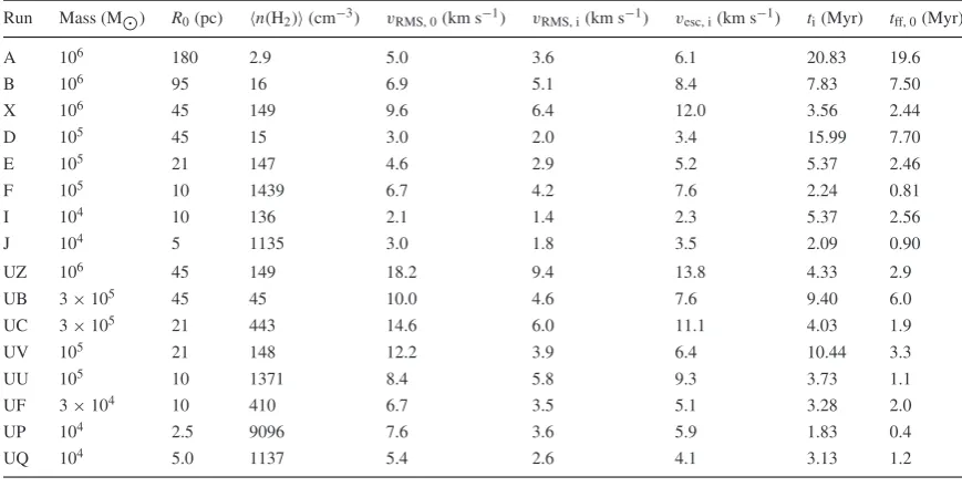
Our initial conditions are the same set of bound and unbound turbulent clouds described in Papers I and III, evolved from the same points in time when each had formed a few massive stars or massive subclusters. In Table1, we summarize the important parameters of all 16 simulations.
3 R E S U LT S
3.1 HIIR morphology
In the lower mass clouds, the winds modify the HIIR morphologies in two ways, depicted in Figs1and2. At early times, the winds
at University of St Andrews on September 5, 2014
http://mnras.oxfordjournals.org/
UC 3×10⁵ 21 443 14.6 6.0 11.1 4.03 1.9
UV 105 21 148 12.2 3.9 6.4 10.44 3.3
UU 105 10 1371 8.4 5.8 9.3 3.73 1.1
UF 3×10⁴ 10 410 6.7 3.5 5.1 3.28 2.0
UP 104 2.5 9096 7.6 3.6 5.9 1.83 0.4
[image:3.595.76.511.93.313.2]UQ 104 5.0 1137 5.4 2.6 4.1 3.13 1.2
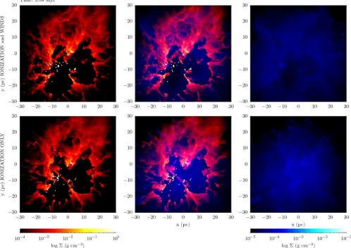
Figure 1. Comparison of the cold gas (left-hand panels) and the HIIRs (right-hand panels) at an early epoch in the Run I calculations with (top row) and without (bottom row) winds included. Centre panels are superpositions of the left- and right-hand panels.
at University of St Andrews on September 5, 2014
[image:3.595.45.541.305.686.2]Figure 2. Comparison of the cold gas (left-hand panels) and the HIIRs (right-hand panels) at the end of the Run UQ calculations with (top row) and without (bottom row) winds included. Centre panels are superpositions of the left- and right-hand panels.
help the HIIRs clear away the dense gas near the massive stars, as illustrated in Fig.1, from Run I. The evacuation of the cold gas (shown in the left-hand panels) is more efficient in the dual-feedback run (top row) than in the ionization-only run (bottom row). This change is reflected in the shape of the HIIR. Dense material near the sources collimates the HIIR in the ionization-only calculation into conical lobes radiating from the central cluster. This morphology is not found in the seminal work of Wood & Churchwell (1989) and is not a typical HIIR shape. However, the clearing away of the collimating material by winds results in a more circular projected morphology. The HIIR at this early epoch would probably be classified as core halo, since it seems to be centrally condensed or multiply peaked.
Later, the winds create large (∼10 pc) holes inside the HIIRs, depicted in Fig.2. This shows the end of the Run UQ calculations, with the ionization-only run at the bottom and the dual-feedback run on top. The HIIR in the ionization-only simulation (lower-right panel) has an irregular morphology and would fall into the centrally condensed or multiply peaked categories of Wood & Churchwell (1989). The wind-blown HIIR (upper-right panel), by contrast, ex-hibits a hole whose shape is roughly the same as, but smaller than, the hole in the cold gas. The top-central panel shows the HIIR as a thick lining of the inner surfaces of the bubbles. This HIIR would probably then be classified as shell-like by Wood & Churchwell (1989). Overall, the action of winds is to suppress the multiple-lobe
morphological type which is not commonly seen, and to generate the shell-like form. From this perspective, the wind-blown HIIRs resemble observed systems better than those created by ionization alone.
We examine the HIIR evolution in more detail by locating the ionization fronts and using their median separation from the bright-est ionizing source to define a bubble radius and volume. Fig.3
shows the ionization-only Run I calculation 0.88 Myr after feed-back was enabled. A column-density projection of the gas is shown in red, orange and yellow. Neutral gas particles located just behind the ionization front(s) are shown as blue dots, the most massive star as a white cross and the median ionization-front radius as a white circle. Note that the true shape of the ionization front is far from spherical.
3.2 HIIR expansion
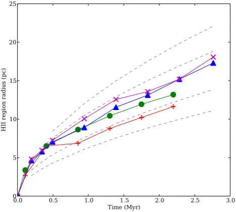
Once the typical ionization-front radius has been defined, we trace the expansion of the HIIR. Fig. 4 shows the time evolution of the median ionization-front radius in the ionization-only and dual-feedback Runs I and UQ.
The evolution of an HIIR in a uniform medium is described by the solution in Spitzer (1978). If the temperature of the ionized gas is fixed, the solution describes a family of curves dependent only on the initial size of the ionized volume, the Str¨omgren radius,
at University of St Andrews on September 5, 2014
http://mnras.oxfordjournals.org/
Figure 3. Render from Run I with gas column density shown in red– orange–yellow colours, particles on the ionization fronts shown as blue dots, the location of the most massive ionizing source shown as a white cross and the bubble defined by the mean distance of all ionization-front particles from the most massive source shown as a white circle.
Figure 4. Evolution of the front radius in the Run I ionization-only (red), dual-feedback (green) and Run UQ ionization-ionization-only (blue) and dual-feedback (magenta) calculations. Representative Spitzer solutions are shown as grey dashed curves.
Rs.Rsis not easy to estimate in inhomogeneous gas, but we plot
for comparison Spitzer evolution curves forRs=1.5, 2.5, 5.0 and
7.5 pc. This allows us to gauge qualitatively the effect of gas leakage and/or winds on the expansion of the HIIRs.
[image:5.595.48.282.58.286.2]The effect of either gas leakage or winds on the bubble expansion appears to be slight Neither process radically alters the expansion laws of the bubbles and the expansion curves do not differ markedly from the Spitzer solution for a closed bubble in a uniform cloud. These results are similar to those obtained by Walch et al. (2012),
Figure 5. Evolution of the pressure inside the 90 (red), 75 (green) and 50 (blue) per cent of the ionized gas closest to the most massive stars in the ionization-only (solid lines) and dual-feedback (dashed lines) Run I calculations.
who modelled the influence of photoionization on fractal clouds. Their fig. 3 shows the evolution of the ionization-front radius for values of the cloud fractal dimensionDin the range 2.0–2.8. They found little change in the evolution with increasing fractal dimen-sion, and the general form of the curves again deviates little from the Spitzer model.
We examine the dynamical influence of the winds in Fig.5, which shows the pressure inside the ionization-only (solid lines) and dual-feedback (dashed lines) HIIRs in Run I as functions of time. At very early times, the pressure in the wind-blown HIIR is roughly an order of magnitude larger, but when the HIIRs break out of the confining cold gas at∼105yr, the pressures rapidly become very
similar.
3.3 HIIR gas leakage
Once we have defined the bubble radius using the median ionization front, we divide the cloud into the ‘bubble’, lying inside the ioniza-tion front, and the ‘cloud’ which lies outside it. We first examine the leakiness of the bubbles to gas. We remove all gas outside them and theionizedgas inside them and perform a Hammer projection from the point of view of the most massive star on the remainder. We then compute the fraction of skynotcovered by neutral gas and thus open to leakage of gas from the bubble.
We show the evolution of these gas leakage factors in Runs I and UQ in Fig.6. The gas leakage factors increase with time as the cold gas is cleared away from the sources. The difference between the ionization-only and dual-feedback calculations is again slight. Gas leakage is small early in the simulations, but increases very rapidly over a few×105yr as the HIIRs burst out of the dense material in
which the O-stars are born. At early times, gas leakage is somewhat larger in the dual-feedback simulations, as the winds initially aid the HIIRs in clearing gas from near the sources. Typical gas leakage factors for these two calculations are 0.6–0.7, whereas for the Run E cloud which is much less severely affected by feedback, the leakage factor is only 0.1–0.2.
Harper-Clark & Murray (2009) constructed one-dimensional models of the Carina nebula in which they pointed out that the model of Weaver et al. (1977) predicts a bubble too large for Carina’s estimated age. They modified the standard model to
at University of St Andrews on September 5, 2014
[image:5.595.46.280.363.573.2]Figure 6. Evolution of the gas leakage factors, the fractions of sky not covered by neutral gas at the front radius, in the Run I ionization-only (red), dual-feedback (green) and Run UQ ionization-ionization-only (blue) and dual-feedback (magenta) calculations.
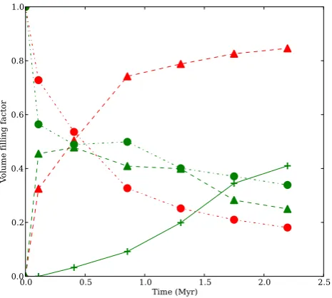
Figure 7. Evolution of the volume-filling factors of HII(triangles and dashed lines), wind (pluses and solid line) and cold neutral gas (circles and dot–dashed lines) within the ionization-front radius in the ionization-only (red) and dual-feedback (green) Run I calculations.
include leakage of wind gas and found that the gas leakage fractions required to achieve agreement with the present state of Carina were
≈0.5, close to the values measured here (note that they discuss the covering factorCf=1−fleak).
3.4 HIIfilling factors
We interpolated the SPH density field on to a grid and counted the fractions of cells inside the ionization front which are filled with HIIor cold gas, or which have been cleared by winds. We show
the time evolution of these filling factors in Run I in Fig.7. In the ionization-only calculation (red lines and symbols), the evolution is
a trade-off between the neutral gas, whose filling factor starts high (as expected for a centrally condensed cloud forming stars near its centre of mass) and falls rapidly to<20 per cent, and the HIIwhich
does the reverse. In a spherical HIIR, one would expect the volume behind the ionization front to be entirely filled by ionized gas, so that the HIIfilling factor would be unity. That this is not so in our
bubbles is a result of the bubbles not being spherical, so that some of the gas behind the median ionization front is actually neutral. However, the bubbles clearly approach a more spherical form as time passes.
In the dual-feedback run, the winds create a cavity inside the HIIR which grows rapidly over∼105yr. The volume-filling factor
of the cavity reaches>40 per cent by the end of the calculation. This correspondingly reduces the filling factor of the ionized gas in the bubble, which rises to≈50 per cent before declining to≈20 per cent. The filling factor of neutral gas in the bubble is higher in the dual-feedback calculation, implying that the bubble has a more complex shape in this calculation. Overall, the filling factors of ionized gas remain large –>10 per cent – in reasonable agreement with the findings of Harper-Clark & Murray (2009).
3.5 Influence of feedback on cold-gas morphology
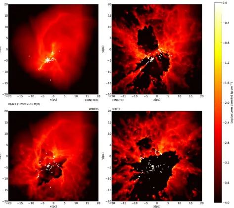
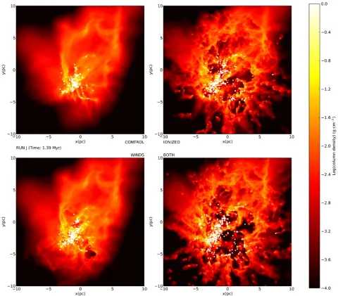
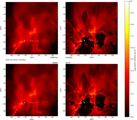
In Figs8–10, we compare the final cold-gas morphology for all four runs of a selection of clouds. The top-left panels show control runs, top-right ionization-only runs, bottom-left winds-only runs and bottom-right winds-and-ionization runs. In general, whether or not winds acting alone were able to strongly influence the morphol-ogy of the clouds, the effects of photoionization clearly dominate at late times in the dual-feedback calculations. The relative effects of winds are strongest at early times when the massive stars are still embedded in very dense gas. Once this gas has been cleared away, the expanding HIIRs assume control of the dynamical and morphological evolution of the clouds.
3.6 Dynamical influence of combined winds and HIIRs
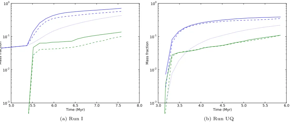
The ability of stellar feedback to expel gas from GMCs is a key issue. We compute at each timestep the fraction of mass in each cloud which has positive total energy in the cloud centre-of-mass frame. Overall, we find that the combined effect of winds and ionization is to unbind substantially more mass than winds acting alone and slightly more than ionization acting alone. Photoionization is a much more destructive agent than winds. Fig.11shows the evolution of the unbound mass fraction (as a fraction of thetotalsystem mass, blue lines) and the ionized gas fraction (as a fraction of the total instantaneous gas mass, green lines) in the ionization-only (dashed lines), winds-only (dotted lines) and dual-feedback (solid lines) Runs I and UQ, these being the bound and unbound clouds with the greatest differences between ionization-only and dual-feedback runs.
The ionization fractions are also generally slightly increased by the action of winds. Where the ionization fraction is noticeably different, the increase occurs early in the simulation, after which the rates of gas ionization in the two calculations are very similar. This is consistent with the picture that winds are effective at early times in clearing away dense gas near the massive stars. However, once this material is destroyed, ionizing photons can penetrate deeper into the gas and the dynamics of the clouds become dominated by photoionization.
In Fig.12, we show the final unbound mass fractions in all bound and unbound clouds as blue (ionization-only), green (winds-only)
at University of St Andrews on September 5, 2014
http://mnras.oxfordjournals.org/
[image:6.595.50.283.332.541.2]Figure 8. Comparison of the cold-gas morphology in the Run I calculations with no feedback (top left), with ionization only (top right), with winds only (bottom left) and with both winds and ionization (bottom right).
and red (dual-feedback) circles plotted over the mass–radius pa-rameter space studied here. We include in the plot the clouds from Heyer et al. (2009) as light grey crosses, contours of cloud escape velocity as dark grey lines and of constant freefall time (and thus volume density) as black lines. There is a clear gradient pointing from high to low escape velocities in the ability of feedback to disrupt clouds. In particular, only clouds whose escape velocity is less than 5 km s−1are significantly damaged, in the sense of having
more than 10 per cent of their mass expelled over the 3 Myr time window.
3.7 Star formation rates and efficiencies
Feedback also affects the star formation process inside clouds. There are various ways in which this may be assessed and this has unfor-tunately led to some rather confusing terminology. In particular, we prefer efficienciesto be dimensionless quantities. For clarity, we here lay out the terms we have used explicitly and explain how we have computed them from our simulations.
(i) The absolute instantaneous star formation rate, [SFR(t)]. This is defined as
SFR(t)= dM∗
dt . (1)
We will approximate the quantity as
SFR(t) =M∗(t)−M∗(t0) (t−t0)
, (2)
wheret0is the time when star formation begins, and we use units
of MMyr−1.
(ii) Theabsolute star formation efficiency, [SFE(t)]. We use this in the sense that it is usually used in star formation and molecular cloud observations and simulations: the fraction of the total mass of system which is stellar at a given time, i.e.
SFE(t)= 1
M∗(t)+Mgas(t)
t
t0
SFR(t)dt= M∗(t)
M∗(t)+Mgas(t)
, (3)
whereM∗(t) andMgas(t) are, respectively, the instantaneous stellar
and gas masses.
at University of St Andrews on September 5, 2014
Figure 9. Comparison of the cold-gas morphology in the Run J calculations with no feedback (top left), with ionization only (top right), with winds only (bottom left) and with both winds and ionization (bottom right).
Matzner & McKee (2000) defined an instantaneous star formation efficiency using the rate dM∗dtat which gas is being converted to stars and the rate dMejdtat which gas is being ejected from the
system in question, as=dM∗/(dM∗+dMej). If the star formation
rates and mass ejection rates do not vary too much over the lifetime of the system, the instantaneous and final star formation efficiencies are nearly the same. However,is only a typical value of the absolute star formation efficiency SFE(t) if both quantities are small. For this reason, and the fact thatdoes not take into account gas which is unbound at the outset of star formation, as in our unbound clouds, we concentrate on the observational quantity SFE(t) here.
(iii) Thestar formation efficiency rate, [SFER(t)]. This is the rate of the change of the star formation efficiency,
SFER(t)= dM∗ dt
1
M∗(t)+Mgas(t)
, (4)
which we approximate by
SFER(t)= [SFE(t)−SFE(t0)] (t−t0)
. (5)
This is what is often measured by galactic and extragalactic studies (e.g. Leroy et al.2008), and is unfortunately often referred to in this context as ‘the star formation efficiency’.
(iv) The star formation efficiency rate per freefall time, [SFERff(t)]. This denotes the change in the star formation efficiency
in one freefall time (e.g. Krumholz & Tan2007; Murray2011), and is equivalent to the star formation rate measured in absolute units multiplied by the local freefall time;
SFER(t)= dM∗ dt
tff
M∗(t)+Mgas(t),
(6)
and is computed by us as
SFERff(t)=
[SFE(t)−SFE(t0)]tff
(t−t0)
. (7)
This quantity is dimensionless.
Since all four quantities listed above may be used to infer dif-ferent things about star formation and difdif-ferent metrics are used by different communities, we plot and discuss them in turn.
at University of St Andrews on September 5, 2014
http://mnras.oxfordjournals.org/
Figure 10. Comparison of the cold-gas morphology in the Run UV calculations with no feedback (top left), with ionization only (top right), with winds only (bottom left) and with both winds and ionization (bottom right).
3.7.1 SFE(t)
Fig. 13 shows the final SFE(tSN) for all runs (tSN= 3 Myr, the
time before the first SN), comparing the control and dual-feedback calculations to assess the ability of feedback to alter the fraction of gas converted to stars over the duration of the simulations. Coloured circles represent the simulation results and grey circles are taken from table 2 in Murray (2011), who investigated 32 GMCs hosting the most luminous star-forming regions in the Milky Way.
The initially unbound control clouds have systematically lower values of SFE(tSN), as also found by Clark et al. (2005). The effect
of feedback on the final stellar masses, denoted by the areas of the red circles relative to the blue, is modest and always negative. The effect tends to be larger for lower mass and lower escape velocity clouds, like the unbound mass fraction. The mean SFE for the bound clouds is reduced by 11 per cent from 0.233 to 0.208, and for the unbound clouds by 22 per cent from 0.125 to 0.098.
Evans et al. (2009) recently measured the SFE of five nearby clouds and found values ranging from 3 to 6 per cent. Thetotal
mass of the five clouds is only≈104 M
, equivalent to one of our runs I, J, UQ or UP, which have final values of SFE(t) of 10– 20 per cent, larger by a factor of around 3.
Murray (2011) investigated clouds with masses in the range 4.3× 10⁴–8.4×10⁶M
which exhibit values of SFE in the range 0.002– 0.273 with a mean of 0.08. They observe a trend of decreasing SFE with increasing cloud mass, but conclude that is likely to be a selection effect. We include their results for comparison and we see that they actually agree rather well.
3.7.2 SFR(t)
In Fig.14, we plot the mean star formation rates over thetSN
feed-back interval for all runs in units of M Myr−1. This quantity
increases with increasing cloud mass, decreases with cloud freefall time and is systematically lower in the initially unbound clouds by factors of a few between clouds of the same mass and size. SFR(t) is also only modestly influenced by feedback. Gravity remains the primary driver of star formation in these simulations.
at University of St Andrews on September 5, 2014
Figure 11. Evolution of the ionized (green lines) and unbound (blue lines) gas fractions in the ionization-only (dashed lines), winds-only (dotted lines) and ionization-and-winds (solid lines) Run I (left) and Run UQ (right)
Figure 12. Fractions of system mass unbound at the ends of the bound-cloud (left) and unbound-cloud (right) simulations, denoted by blue (ionization-only), green (winds-only) and red (dual-feedback) circles.
In their≈104M
total-mass sample of nearby molecular clouds, Evans et al. (2009) measure a total SFR(t) of 256 M Myr−1.
This rate is actually very close to that seen in runs I, UQ and UF which perhaps suggests that the observed clouds may achieve comparable SFE(t) to these simulations in the future. Evans et al. (2009) remark that the star formation rates in their sample would result in SFE(t) reaching values of 15–30 per cent if they persisted for another 10 Myr.
3.7.3 SFER(t)
We plot the star formation efficiency rate SFER(t) in units of Myr−1
in Fig.15. This quantity varies little with cloud mass but increases
substantially with decreasing cloud freefall time. SFER(t) is consid-erably smaller in the initially unbound clouds, having typical values of a few per cent Myr−1, whereas it reaches≈10 per cent Myr−1for
bound clouds with freefall times of 1 Myr. Feedback clearly reduces SFER(t) significantly for several of the smaller model clouds.
It is instructive to compare these values with the survey of SFER(t) in 23 nearby galaxies in Leroy et al. (2008). They compute SFER(t) as
SFER(t)obs=
SFR
gas
, (8)
where SFR is the star formation rate surface density
in MMyr−1pc−2and
gasis the gas surface density in Mpc−2.
The typical gas surface densities for the molecule-dominated
at University of St Andrews on September 5, 2014
http://mnras.oxfordjournals.org/
[image:10.595.52.546.308.545.2]Figure 13. SFE at the ends of the bound-cloud (left) and unbound-cloud (right) simulations, denoted by blue (control runs) and red (dual-feedback runs) circles. Results from Murray (2011) are shown as grey circles.
Figure 14. Mean values of SFR over the feedback interval for the bound-cloud (left) and unbound-cloud (right) simulations, denoted by blue (control runs) and red (dual-feedback runs) circles.
regions of the spirals in their sample are a few×10 Mpc−2and
for the dwarfs an order of magnitude less.
They obtain typical values of SFER(t) in regions of spiral galaxies where the gas mass is largely molecular of∼5×10⁻⁴Myr−1(they
obtain a similar typical value for dwarf galaxies where the ISM mass is dominated by HI). This quantity is∼102times smaller than
the values of SFER(t) we compute here. However, the observed values are likely to be decreased by the dilution of star-forming gas in the telescope beams with non-star-forming material, raisinggas
relative toSFR.
Evans et al. (2009) discuss their results in light of this issue. For their sample of low-mass clouds, they obtain SFER(t) of 3–6 per cent over the last 2 Myr, corresponding to 1.5−3 per cent Myr−1,
com-parable to the lower range of values we measure. However, we note that they define the borders of their clouds as theAV=2 contour,
corresponding to≈6×10⁻³g cm−3. Using the same criterion for
our own clouds would reduce by factors of a few to 10 the quantities of non-star-forming gas and thus increase the apparent SFE by the same factor. We therefore conclude that our clouds are forming stars a factor of at least a few too quickly.
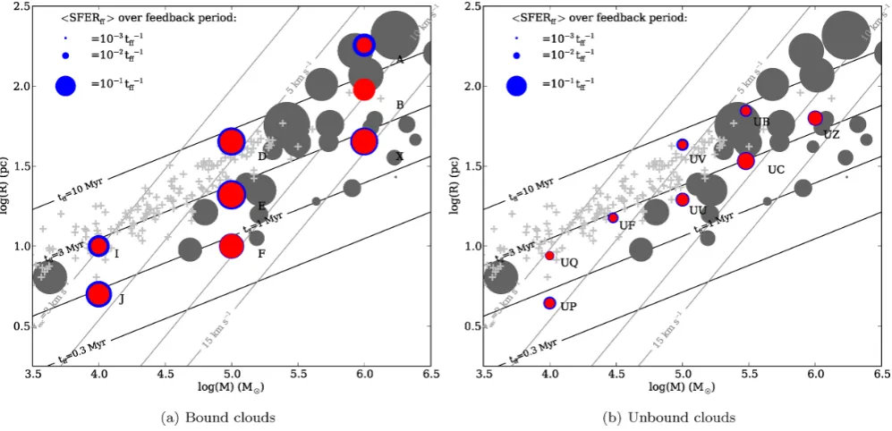
at University of St Andrews on September 5, 2014
[image:11.595.45.545.337.581.2]Figure 15. Mean values of SFER(t) over the feedback interval for the bound-cloud (left) and unbound-cloud (right) simulations, denoted by blue (control runs) and red (dual-feedback runs) circles.
Figure 16. Mean values of SFERff(t) over the feedback interval for the bound-cloud (left) and unbound-cloud (right) simulations, denoted by blue (control
runs) and red (dual-feedback runs) circles. Results from Murray (2011) are shown as grey circles. 3.7.4 SFERff(t)
Finally, in Fig.16, we plot SFERff(t), again including the data from
Murray (2011). This plot shows that, in general, the initially un-bound clouds convert gas to stars more slowly and the cloud un- bound-edness is the dominant parameter determining SFERff, although
feedback does have some influence. SFERffis nearly constant in
the bound clouds at values of the order of 10 per cent and nearly constant in the bound clouds at values of around 3 per cent.
Krumholz & Tan (2007) measured SFERff(t) in a variety of
sys-tems of different densities and inferred typical values of≈0.02,
essentially independent of density [although see Elmegreen (2007) for further discussion of these measurements]. Evans et al. (2009) obtain values of SFERff(t) in the range 0.03–0.06, for entire clouds,
but rather larger values (0.1–0.25) for dense cores. The values of SFERff(t) computed by Murray (2011) are generally larger than
those in our unbound clouds, but are comparable in the case of the bound clouds. Their observed values are in the range 0.001–0.592 with a mean of 0.16.
In our bound clouds, the mean SFERff(t) is reduced by feedback
by 29 per cent from 0.160 to 0.113 and in the unbound clouds by
at University of St Andrews on September 5, 2014
http://mnras.oxfordjournals.org/
[image:12.595.49.548.340.581.2]of the evolution. The lower mass clouds in particular lose substantial fractions (0.5–0.9) of their ionizing photons. A similar degree of photon loss was reported by Walch et al. (2012) in their studies of the disruption of 104M
fractal clouds.
In Fig.17, we plot effective ionizing luminosities for each cloud. Although the clouds’ actual fluxes and photon leakage fractions vary considerably, they do so in opposite directions, so that the effective fluxes (with the exception of the strongly gas-depleted Run F) fall in a narrow range. The more massive and denser clouds tend to have higher absolute luminosities because of their higher star formation efficiencies. These are also the clouds least affected by feedback and therefore least likely to lose photons. There is a clear trend for the bound clouds to be more luminous, in absolute and effective terms, than the unbound clouds because of their higher SFEs. In general, all clouds (save Run F) have an effective luminosity close to 1049s−1.
Run F is bright because of its very high star formation efficiency and it being close to gas exhaustion by the end of the feedback time window. Such behaviour is expected of starburst clouds.
3.9 Transparency to SN ejecta
Fig.18depicts the fraction of the ejecta from the first SN explosion in each cloud which is expected to escape. This was computed in the same fashion as in Papers I and III.
All but the most massive clouds will leak substantial fractions of their first SN ejecta. Conversely, while a few of the lowest mass clouds – Run I, J and UQ – will be essentially destroyed by their first SN, large quantities of material in the more massive and denser clouds are likely to survive. It is therefore possible that there will be a second round of star formation involving debris-polluted gas in these clouds. This is especially true of the more massive clouds which will likely be able to withstand several SN explosions, as is the case in the 30 Doradus region (Townsley et al.2006, and references therein).
4 D I S C U S S I O N
4.1 Effects of HIIRs versus winds
Our treatment of stellar winds as purely sources of momentum is plainly simplified and limits the range of phenomena that we can observe. Since we do not inject hot wind gas into our calculations, we do not correctly model interactions between the wind and the molecular material such as Kelvin–Holmholtz instabilities or ther-mal/hydrodynamical ablation of cold material by the hot wind. This limits the ability of our winds to entrain material from the clouds.
the shocked stellar wind is able to cool maximally effectively. The thermodynamics of wind bubbles interacting with HIIRs are in reality more complex. This issue was recently studied in one-dimensional simulations by Martinez-Gonzalez, Silich & Tenorio-Tagle (2014). There is always an initial period during which the wind remains hot and the pressure in the wind bubble within the HIIR is very high. This drives a shock into the ionized gas, sweeping up an ionized shell. If this shell becomes sufficiently dense, recom-binations within it may consume all of the O-stars’ ionizing flux, trapping the HIIR inside the wind bubble. However, the duration of this phase depends strongly on the ability of the wind to cool. There are two major mechanisms which are likely to control when this occurs: evaporation from the inner wall of the ionized shell and mass loading from ablation/evaporation of dense cold clumps inside the wind bubble.
The former was considered by Mac Low & McCray (1988) who computed a cooling time for the bubble (their equation 14). This time-scale is short (∼105yr) for most of our simulations, although ∼1 Myr for a few of our largest, lowest density clouds such as Run A, if they are treated as a single bubble and not as several interacting bubbles.
There are numerous small cold clumps inside our HIIRs and wind bubbles, and photoevaporation of these objects would further mass load a real wind and shorten its cooling time further. We compared their evaporation time-scales in the simulations to those given by Pittard (2007) and references therein and find good agreement, indi-cating that these and other photoevaporative flows in the simulations are adequately resolved. In common with Rogers & Pittard (2013), we find that these objects are rather long-lived, often surviving for
∼1 Myr. Their contribution to mass loading would be small com-pared to thermal evaporation at the edge of the wind bubble, as estimated by Mac Low & McCray (1988).
We conclude that momentum-dominated winds are a reasonable assumption for the embedded clusters modelled here and observe that they are a rather small perturbation on the effects of the HIIRs. Our findings that the winds are confined by the HIIRs are in agree-ment with those of several other authors (e.g. McKee et al.1984; Krumholz & Matzner2009; Yeh & Matzner2012).
We alluded briefly to this issue in Paper V where we simply compared in Fig.9the expansion laws of momentum-driven wind bubbles and HIIRs and showed that, except at very early times or ex-treme densities, the HIIR was always larger. We here give a slightly more sophisticated analysis. We consider a wind bubble expanding into an HIIR. The HIIR has radiusrII(t), densityρII(t), pressure PII(t) and internal sound speedcII=10 km s−1. The wind bubble
has radiusrw(t)<rII(t). The driving star has an ionizing photon flux
at University of St Andrews on September 5, 2014
Figure 17. Effective Lyman continuum luminosities for the bound-cloud (left) and unbound-cloud (right) simulations, denoted by red (control runs) and blue (dual-feedback runs) circles.
Figure 18. Fraction of ejecta lost from first SN for the bound-cloud (left) and unbound-cloud (right) simulations, denoted by red (control runs) and blue (dual-feedback runs) circles.
QH=1049s−1, a wind mass-loss rate ˙M=10−6Myr−1and a
wind terminal velocityv∞=2000 km s−1, and the original neutral
medium has a mass densityρ0and a number densityn0. At timet,
the radius of the unperturbed HIIR is given by
rII(t)=Rs
1+ 7
4
cIIt
Rs
4 7
(9)
(Spitzer1978) and the pressure by
PII(t)=ρII(t)c2II=ρ0
1+7
4
cIIt
Rs
−6 7
c2
II (10)
(Bisbas et al.2009), where the pressure is assumed to be uniform, andRsis the Str¨omgren radius,
Rs=
3QH
4πn2 0αB
1 3
. (11)
We now make the simple assumption that a wind bubble expands inside the HIIR until the ram pressure atrwis equal to the pressure
inside the HIIR, which is modified from its unperturbed valuePII
at University of St Andrews on September 5, 2014
http://mnras.oxfordjournals.org/
[image:14.595.49.545.331.575.2]Figure 19. Evolution of the ratio of the wind bubble radius to the HIIR radius as a function of time for four values ofn0as computed from equation
(15) (coloured lines) and as measured in Run UQ (black line).
to a new valuePII, was
PII,w=PII
r3 II
(rII−rw)3
. (12)
The effects of the winds are assumed not to alter the radius of the HIIR or the ionized gas mass. We may then equate the pressures and, after some rearrangement, we arrive at
1
r2 w
= rII3
(rII−rw)3
4πρ
0c2II
˙
Mv∞
1+7 4
cIIt
Rs
−6 7
= rII3
(rII−rw)3
β(t). (13)
If we assume thatr<rII, we are justified in taking only the first two
terms in the expansion of (rII−rw)3and we obtain an expression
forrw:
r2 w+
3rw
β(t)rII(t)
− 1
β(t) =0. (14)
We plot the evolution of this function for several values ofn0 in
Fig.19. Since the initial pressure of the HIIR scales withn0, the
ra-tiorw/rIIincreases with decreasingn0. However, the wind bubble is
always substantially smaller than the HIIR. Yeh & Matzner (2012) define a parameter =Pwrw3/(PIIrII3−Pwrw3) to quantify the
im-portance of winds in HIIRs. The models presented above have in the range 0.1–1 The influence of radiation pressure (discussed below) is likely to be small, so these models fall into the class of classical Str¨omgren HIIRs (see fig. 1 in Yeh & Matzner2012).
The above analysis applies to a spherical non-leaking bubble. In a leaky bubble, the pressure inside the HIIR drops much faster than it would otherwise, which allows the wind bubble to expand to occupy a greater proportion of the HIIR interior. We also plot in Fig.19the time evolution ofrw/rIImeasured in Run UQ. This
calculation’s initial number density is≈103cm−3, but the evolution
ofrw/rIIis closer to that of a cloud withn0=10 cm−3.
The two principal influences of photoionization on the cold gas – ionization of fresh material and the thermal pressure of the HIIR on the inner walls of the bubbles – are not much influenced by the winds in our calculations. Although the ionized gas morphology and
The influence of feedback on the global evolution of our model clouds was generally modest. The quantities of gas actually ion-ized are small and do not vary a great deal amongst calculations, generally being 3–10 per cent. Typical photoevaporation rates are
∼10−2M
yr−1for the 106M
clouds and∼few×10−3M yr−1
for the 105 and 104 M
clouds, so do not vary very much with cloud mass. They are lower in clouds with larger escape velocities for a given mass.
Several authors have examined this problem analytically (e.g. Whitworth1979; Williams & McKee1997). Matzner (2002) de-rived the following expression relating the quantity of matter pho-toevaporated,δMdest, to the ionization time-scalet, cloud column
densityNH2and massMc, and the total ionizing luminosityQH:
δMdest=1.2×10⁴M
t
3.7 Myr 9
7 N
H2
1.5×1022cm−2
−3 14
×
M
c
106M
1
14 Q
H
1049s−1
4 7
. (15)
This expression is strictly only valid for blister HIIRs and the anal-ysis which generated it ignores both gravity and cloud internal structure. However, comparing with the quantities of gas photoion-ized in our simulations (to be strictly consistent, we compared with our ionization-only calculations, but these differ little from the dual-feedback simulations presented here), we find rather good agreement, usually within a factor of 2. Equation (15) predicts less photoevaporation for clouds with low and intermediate escape ve-locities (the largest discrepancy being by a factor of 4.5 for Run D), and more for clouds with high escape velocities, the largest discrepancy being by a factor of 2.6 for Run X. As well as being in reasonable consensus, the trend in the discrepancies points in the expected direction in that the clouds with the highest escape velocities, where gravity plays a greater role, are those for which equation (15) overestimates the ionized mass.
Krumholz, Matzner & McKee (2006) and Goldbaum et al. (2011) perform one-dimensional simulations of the effects of HIIRs on clouds over much longer time-scales than we are able to address here. Krumholz et al. (2006) find that 50–70 per cent of their 2×10⁵and 1×10⁶M
clouds are evaporated on time-scales of 10 and 20 Myr, respectively, which implies an average of 7– 10 per cent per 3 Myr. These rates are larger than we observe but again not by very large factors, at most around 5. Goldbaum et al. (2011) find average photoevaporation rates in their accreting-cloud models of the order of 10−2M
yr−1, comparable to our
106M
clouds but factors of 3–5 larger than our 105M
clouds.
at University of St Andrews on September 5, 2014
[image:15.595.307.544.384.443.2]These calculations involve gravity but do not account for photon leakage or inhomogeneities in the gas structure, which may explain why we observe smaller photoevaporated masses. In general, our results agree with the above-cited works that the destruction time-scales for large GMCs can be long. Given that we expect such clouds to also survive several SN, our results also allow cloud lifetimes of 10–20 Myr.
Only the lower density and lower mass clouds had substantial fractions of their mass unbound overtSN. The amount of material
unbound is controlled by the cloud escape velocity relative to the fixed ionized sound speed.
Changes in the star formation rates and efficiencies were negative but slight – never as much as a factor of 2, even for the low-mass clouds most severely damaged by feedback. Clouds formed stars on approximately their freefall time-scales. Both of these results suggest that feedback is largely unable to wrest control of the clouds from gravity.
V´azquez-Semadeni et al. (2010) find that their HII-region like
feedback is not very effective indestroyingtheir model clouds, al-though they found that it could be destructive on smaller scales. This is in general agreement with our results – feedback is able to destroy small- and medium-scale structures, but generally struggles to dis-mantle the largest clouds. These findings are broadly in agreement with those of V´azquez-Semadeni et al. (2010) and Walch et al. (2012), who also find that photoionization is damaging to lower mass (∼104M
) clouds. Semi-analytic models by Krumholz et al. (2006) also concluded that lower-mass clouds should survive for shorter times than the largest clouds.
In Table 2, we compare the star formation efficiencies, rates, efficiency rates and efficiency rates per freefall time in our dual-feedback models with those of Krumholz & Tan (2007), Evans et al. (2009) and Murray (2011). Our model clouds form stars too fast and too efficiently by most measures by factors of a few. Feedback has only a modest influence on the rate and efficiency of star formation. These results contrast somewhat with those of V´azquez-Semadeni et al. (2010). They studied the effects of stellar feedback on flattened molecular clouds formed by colliding flows. They found that, depending on the size scales of substructure in the clouds, the SFE was reduced by factors of 3–10. They use a slightly different definition of SFE from us; SFE=M∗/(Mdense+M∗), whereMdense
is the mass of gas whose density exceeds 50 cm−3. They observe
that feedbackincreasesthe quantity of dense gas whiledecreasing the stellar mass. This, combined with the definition of SFE given above, makes the amplitude of variation of the SFE larger than what we measure here, using thetotalgas mass, although not by large factors. It is not clear to us why feedback has a substantially greater influence on star formation in V´azquez-Semadeni et al. (2010)’s calculations, although it may be related to the flattened geometry of their clouds. We will discuss this issue in greater detail in a companion paper.
There is an additional reason why the final stellar masses of our denser clouds tend to be less affected by feedback. Since we have assumed that feedback is driven purely by O-stars and all our calculations start from starless clouds, each cloud must first form O-stars before feedback can act. O-stars or O-star-bearing clusters take time to form and each cloud continues to form lower mass stars/clusters in the meantime. Clouds which overall have higher fractional rates of conversion of mass to stars (i.e. higher values of SFER(t)) are likely to have converted more of their gas reserves to stars before forming their first O-stars and to therefore be more difficult to unbind. We again defer a detailed discussion of this issue to a later paper.
4.3 Neglected physical effects
In these calculations, we have neglected some important physics, particularly the following.
(i) Small-scale feedback such as jets and outflows and thermal feedback from accretion on to protostars which should reduce the local star formation efficiency by factors of a few. Matzner & McKee (2000) examined the influence of momentum input from outflows on the formation of low-mass clusters and concluded that they were able to restrain the star formation efficiencies to values of 30– 50 per cent. Thermal feedback from protostellar accretion affects the fragmentation process (e.g. Matzner & Levin2005; Stamatellos, Hubber & Whitworth 2007). Price & Bate (2009) modelled this process on the scale of a small cluster. They found that it limited fragmentation on small scales, reducing the numbers of stars formed and the total stellar mass by factors of up to a few. This issue can also be approached by asking whether multiple outflows drive turbulence, which supports clouds against collapse on large scales. Li & Nakamura (2006), Nakamura & Li (2007) and Matzner (2007) all concluded that outflows can be efficient drivers of turbulence. Wang et al. (2010) modelled the influence of magnetic fields and outflows on the star formation rates in turbulent cores. They showed that they have complementary effects, together decreasing SFRs by a factor of approximately 3 over time-scales of∼1tff.
(ii) Magnetic fields, which are likely to depress the overall rate of star formation on large and small scales. Numerous recent studies (e.g. Price & Bate2009; Wang et al.2010; Padoan & Nordlund
2011; Peters et al.2011; V´azquez-Semadeni et al.2011; Federrath & Klessen2012; Myers et al.2014) have found that the support pro-vided at intermediate and large scales by magnetic fields slows star formation rates by factors of a few up to an order of magnitude in the case of V´azquez-Semadeni et al. (2011). The interaction of HIIRs with magnetic fields has been less intensively studied. Krumholz, Stone & Gardiner (2007b) and Peters et al. (2011) both find that magnetic fields constrain the expansion of HIIRs, at least in some directions. Gendelev & Krumholz (2012) find that that the presence of magnetic fields results in a much larger injection of energy into the cold gas, although much of the additional energy is stored in the magnetic field. Arthur et al. (2011) came to a similar conclusion in their simulations of magnetizsed HIIRs growing around O- and B-stars, finding that large quantities of energy were stored in the magnetic fields, but that the differences in bubble evolution were modest.
(iii) Radiation pressure, which has effects similar to stellar winds but is rather more difficult to model. A star’s total radiative momen-tum flux ˙pRADis given byLbol/c, whereLbolis the star’s bolometric
luminosity. The stars’s wind momentum flux ˙pWINDis ˙Mv∞, where
˙
Mis the wind mass-loss rate andv∞is its terminal velocity. Given expressions that describe the bolometric luminosity, mass-loss rate and wind terminal velocity as functions of mass, the relative con-tribution of radiation pressure and winds from a given star may be computed. Here we takeLbol(M) to be given by
Lbol(M)=(M/M)4L M <2 M
0.73(M/M)3.5L
2< M <20 M 1140(M/M) L 20 M< M
(16)
(Fall, Krumholz & Matzner2010). The functions used to compute the wind mass-loss rates and terminal velocities are given in Paper V as
˙
M(M∗)=
0.3 exp
M∗
28
−0.3
×10−6Myr−1 (17)
at University of St Andrews on September 5, 2014
http://mnras.oxfordjournals.org/
and
v∞(M∗)=103(M∗−18)0.24+600km s−1. (18)
We neglect in these calculations feedback from all stars less massive than 20 M, and no star more massive than 65 Mexists in any simulation. Evaluating the ratio ˙pRAD/p˙WINDfor these stars gives
0.82 and 0.18, respectively, since the wind momentum declines steeply towards lower masses, whereas the radiation momentum varies linearly with mass. The stars with the largest momentum flux, which dominate the total flux, are therefore those for which radiation pressure would make the smallest relative contribution. Overall, radiation pressure is a perturbation of order unity to the wind momenta for individual stars in this mass range. This quantity can be straightforwardly integrated over the stellar mass function, adequately described by a Salpeter function between 0.5 and 65 M for simulations in which we resolve stars, and a similar function for those in which we can only resolve clusters. If we again ignore winds entirely for stars less massive than 20 Mbut include the ra-diation pressure from all stars, the total radiative momentum flux is
≈50 per cent larger than the total wind flux. However, this still rep-resents a correction of order unity which is unlikely to substantially influence our results.
Sales et al. (2014) simulated the effects of direct radiation pressure and/or photoionization on uniform and isothermal-profile clouds. They found that radiation pressure was able to accelerate large quantities of gas to high velocities, but took a long time to do so. If photoionization was also active, it was much more rapidly acting and tended to dominate.
In common with Sales et al. (2014), we have neglected in the above analysis multiple photon scatterings, which increases the coupling of the radiative momentum flux to the gas by a factor termed ftrap by Krumholz & Matzner (2009), who argue that its
value should be ≈2. However, in protocluster clouds with large optical depths (i.e. with large surface – but not necessarily volume – densities),ftrapcan be larger. Fall et al. (2010) takeftrap=2–5 and
argue that radiation pressure from massive (>104M
) clusters in dense ( >a few×10−2–10−1g cm−2) clouds dominates over all
other feedback mechanisms. Murray, Quataert & Thompson (2010) argue in a similar fashion and present models of W49 and G298.4-0.3, which have surface densities in the range 0.05–0.1 g cm−2,
showing that radiation pressure forces are always larger than HII
gas pressure forces.
While very few individual subclusters in our simulations reach 104M
, the total stellar mass in many of our large clouds exceeds this value and some clouds (e.g. Runs X and F) have surface densi-ties in the regime where these authors find radiation pressure to be
important. It is therefore possible that radiation pressure would be significant in some of our models, and we will address this issue in future work.
4.4 Leakage of photons from HIIRs
The loss of ionizing photons by massive star-forming regions is a key ingredient in three major areas of astrophysics, namely the en-ergetics of the large-scale ISM, the inference of star formation rates in unresolved stellar populations (for example, in dwarf galaxies) and the reionization of the Universe.
The source of photons required to maintain the diffuse ionized gas in spiral galaxies is still a matter of debate, but there seems to be a consensus that O-stars are responsible for most of it but that the contribution of field O-stars is not sufficient, so that em-bedded massive stars must make up much of the difference (Voges & Walterbos2006). This in turn requires that the clouds in which these stars are embedded are porous to photons. Whether this is the case can only be addressed by GMC-scale simulations of the kind presented here. This issue has been addressed before using, for example, ionizing sources in static fractal density distributions (e.g. Wood et al.2005) but it is only relatively recently that esti-mates could be self-consistently made from dynamical simulations in which the dynamics is largely driven by ionization itself (e.g. Walch et al.2012).
We found that all of our clouds, with the exception of the severely gas-depleted Run F, leak ionizing photons at close to the same rate of∼1049 s−1regardless of mass. Their specific effective ionizing
luminosities are therefore proportional toM−1
cloud. This in turn implies
that, for any cloud mass function where there are more low-mass clouds than high-mass clouds, such as in M33 (Engargiola et al.
2003), most of the photons ionizing the ISM originate from low-mass clouds.
The questions of inferring stellar IMFs and star formation histo-ries from the emission of massive stars and of reionization of the Universe are concerned with the issue of the escape of photons from galaxies. Gnedin, Kravtsov & Chen (2008) for example use an AMR simulation with minimum comoving resolutions of≈50 pc to study the escape of ionizing photons from high-redshift galaxies, com-puting source luminosities using STARBURST99 (Leitherer et al.
1999). This resolution limit is roughly the size of a whole GMC and therefore cannot include the physics in our calculations, which would modify the emission of clusters from the STARBURST mod-els. The simulations presented here may therefore be useful as sub-grid inputs for large-scale calculations.
at University of St Andrews on September 5, 2014
[image:17.595.144.448.83.193.2]5 C O N C L U S I O N S
In this and preceding papers, we have examined the evolution of a set of 16 model GMCs characterized by radius, mass and initial turbu-lent velocity dispersion under four different physical assumptions: they suffer no feedback at all from their stars, that they experi-ence ionizing radiation only, that they experiexperi-ence winds only or that they experience both forms of feedback. Modulo the simplifying assumptions we have made about modelling the feedback, we are now in a position to draw some conclusions about the relative and total influence of winds and photoionization.
(i) Except at very early times when the OB-stars are still deeply embedded, the dynamical effects of the two forms of feedback are dominated by photoionization. The additional influence of the winds on the cold gas and on the star formation process is essentially a perturbation.
(ii) Winds are able to substantially modify the morphology of theionizedgas in two ways. At early stages of the cloud evolution, when the HIIRs are still breaking out of the dense filamentary gas where the O-stars are located, winds help clear the gas away and reduce collimation of the ionized flows. This produces roughly spherical HIIRs more closely resembling common morphological types observed by Wood & Churchwell (1989) than the multilobed structures seen in the ionization-only calculations.
At later stages, the wind-blown HIIRs often exhibit central holes with typical sizes∼10 pc, closely corresponding to the shell-like morphological class identified by Wood & Churchwell (1989). Overall, the shapes of the wind-blown HIIRs are more realistic than those from the ionization-only simulations.
(iii) As with ionization acting alone, the combined effects of winds and ionization on the cloud dynamics can be substantial when compared with the absence of any feedback. In the 3 Myr time window before the first SN are expected, winds and ionization are able in some cases to unbind more than half the mass of their host clouds. However, the degree of influence is strongly constrained by the clouds’ escape velocities. While feedback is very destructive to the lower mass and lower density clouds modelled here, it has very little effect on the more massive and denser objects.
(iv) The influence of winds and ionization on star formation rates, efficiencies and efficiency rates is rather modest. In particular, the mean final SFEs of the bound and unbound clouds are reduced by 11 and 22 per cent, respectively, to mean values of 0.1–0.2. Mean SFERff’s are reduced by around one third in both cloud samples to
values of 3–11 per cent. By most measures, the clouds form stars too fast and too efficiently in general, and feedback does relatively little to change this picture.
(v) The model clouds leak substantial quantities of ionizing pho-tons. The leakiness and intrinsic luminosity anticorrelate so that the effective luminosities of the clouds are nearly independent of mass at a few×1049s−1.
(vi) Most of the clouds are also leaky with respect to SN debris and all except the lowest-density low-mass clouds are likely to survive at least one SN explosion.
(vii) As well as photons, the HIIRs are also permeable to their own ionized gas. The fact that the HIIRs are leaky strongly affects the dynamics of the bubbles and limits the amount of damage they can do to their host clouds.
AC K N OW L E D G E M E N T S
We thank the referee, Chris Matzner, for very interesting com-ments and suggestions which resulted in a more comprehensive
manuscript. This research was supported by the DFG cluster of excellence ‘Origin and Structure of the Universe’ (JED, BE). IAB acknowledges funding from the European Research Council for the FP7 ERC advanced grant project ECOGAL. JN would like to acknowledge the German Deutsche Forschungsgemeinschaft, DFGPR 569/9-1.
R E F E R E N C E S
Agertz O., Kravtsov A. V., Leitner S. N., Gnedin N. Y., 2013, ApJ, 770, 25 Arthur S. J., Henney W. J., Mellema G., de Colle F., V´azquez-Semadeni E.,
2011, MNRAS, 414, 1747 Bate M. R., 2009, MNRAS, 392, 1363
Bate M. R., Bonnell I. A., Price N. M., 1995, MNRAS, 277, 362 Bisbas T. G., W¨unsch R., Whitworth A. P., Hubber D. A., 2009, A&A, 497,
649
Capriotti E. R., Kozminski J. F., 2001, PASP, 113, 677
Clark P. C., Bonnell I. A., Zinnecker H., Bate M. R., 2005, MNRAS, 359, 809
Cunningham A. J., Klein R. I., Krumholz M. R., McKee C. F., 2011, ApJ, 740, 107
Dale J. E., Bonnell I. A., 2008, MNRAS, 391, 2
Dale J. E., Bonnell I. A., Clarke C. J., Bate M. R., 2005, MNRAS, 358, 291 Dale J. E., Ercolano B., Clarke C. J., 2007, MNRAS, 382, 1759
Dale J. E., Ercolano B., Bonnell I. A., 2012a, MNRAS, 424, 377 (Paper I) Dale J. E., Ercolano B., Bonnell I. A., 2012b, MNRAS, 427, 2852
(Paper II)
Dale J. E., Ercolano B., Bonnell I. A., 2013a, MNRAS, 430, 234 (Paper III) Dale J. E., Ercolano B., Bonnell I. A., 2013b, MNRAS, 431, 1062
(Paper IV)
Dale J. E., Ngoumou J., Ercolano B., Bonnell I. A., 2013c, MNRAS, 436, 3430 (Paper V)
Elmegreen B. G., 2007, ApJ, 668, 1064
Engargiola G., Plambeck R. L., Rosolowsky E., Blitz L., 2003, ApJS, 149, 343
Evans N. J., II et al., 2009, ApJS, 181, 321
Fall S. M., Krumholz M. R., Matzner C. D., 2010, ApJ, 710, L142 Federrath C., Klessen R. S., 2012, ApJ, 761, 156
Fierlinger K. M., Burkert A., Diehl R., Dobbs C., Hartmann D. H., Krause M., Ntormousi E., Voss R., 2012, in Capuzzo-Dolcetta R., Limongi M., Tornamb`e A., eds, ASP Conf. Ser. Vol. 453, Advances in Computational Astrophysics: Methods, Tools, and Outcome. Astron. Soc. Pac., San Francisco, p. 25
Freyer T., Hensler G., Yorke H. W., 2003, ApJ, 594, 888 Freyer T., Hensler G., Yorke H. W., 2006, ApJ, 638, 262 Gendelev L., Krumholz M. R., 2012, ApJ, 745, 158
Gnedin N. Y., Kravtsov A. V., Chen H.-W., 2008, ApJ, 672, 765
Goldbaum N. J., Krumholz M. R., Matzner C. D., McKee C. F., 2011, ApJ, 738, 101
Gritschneder M., Naab T., Walch S., Burkert A., Heitsch F., 2009, ApJ, 694, L26
Hansen C. E., Klein R. I., McKee C. F., Fisher R. T., 2012, ApJ, 747, 22 Harper-Clark E., Murray N., 2009, ApJ, 693, 1696
Heyer M., Krawczyk C., Duval J., Jackson J. M., 2009, ApJ, 699, 1092 Hopkins P. F., Keres D., Onorbe J., Faucher-Giguere C.-A., Quataert E.,
Murray N., Bullock J. S., 2013, preprint (arXiv:e-prints) Krumholz M. R., Matzner C. D., 2009, ApJ, 703, 1352 Krumholz M. R., Tan J. C., 2007, ApJ, 654, 304
Krumholz M. R., Matzner C. D., McKee C. F., 2006, ApJ, 653, 361 Krumholz M. R., Klein R. I., McKee C. F., 2007a, ApJ, 656, 959 Krumholz M. R., Stone J. M., Gardiner T. A., 2007b, ApJ, 671, 518 Krumholz M. R., Cunningham A. J., Klein R. I., McKee C. F., 2010, ApJ,
713, 1120
Krumholz M. R., Klein R. I., McKee C. F., 2012, ApJ, 754, 71 Leitherer C. et al., 1999, ApJS, 123, 3
Leroy A. K., Walter F., Brinks E., Bigiel F., de Blok W. J. G., Madore B., Thornley M. D., 2008, AJ, 136, 2782
at University of St Andrews on September 5, 2014
http://mnras.oxfordjournals.org/
Pellegrini E. W., Baldwin J. A., Ferland G. J., 2011, ApJ, 738, 34 Peters T., Mac Low M., Banerjee R., Klessen R. S., Dullemond C. P., 2010,
ApJ, 719, 831
Peters T., Banerjee R., Klessen R. S., Mac Low M.-M., 2011, ApJ, 729, 72 Pittard J. M., 2007, in Hartquist T. W., Pittard J. M., Falle S. A. E. G., eds, Astrophysics and Space Science Proc., Diffuse Matter from Star Forming Regions to Active Galaxies – A Volume Honouring John Dyson. Springer, Dordrecht, p. 245
Price D. J., Bate M. R., 2009, MNRAS, 398, 33 Rogers H., Pittard J. M., 2013, MNRAS, 431, 1337
Sales L. V., Marinacci F., Springel V., Petkova M., 2014, MNRAS, 439, 2990
Westmoquette M. S., Dale J. E., Ercolano B., Smith L. J., 2013, MNRAS, 435, 30
Whitworth A., 1979, MNRAS, 186, 59 Williams J. P., McKee C. F., 1997, ApJ, 476, 166 Wood D. O. S., Churchwell E., 1989, ApJS, 69, 831
Wood K., Haffner L. M., Reynolds R. J., Mathis J. S., Madsen G., 2005, ApJ, 633, 295
Yeh S. C. C., Matzner C. D., 2012, ApJ, 757, 108
This paper has been typeset from a TEX/LATEX file prepared by the author.
at University of St Andrews on September 5, 2014