(will be inserted by the editor)
Computational modelling of cancer development and
growth: Modelling at multiple scales and multiscale
modelling
Zuzanna Szyma´nska · Maciej Cytowski ·
Elaine Mitchell · Cicely K. Macnamara ·
Mark A.J. Chaplain
Received: date / Accepted: date
Abstract In this paper we present two mathematical models related to differ-ent aspects and scales of cancer growth. The first model is a stochastic spatio-temporal model of both a synthetic gene-regulatory network (the example of a three-gene repressilator is given) and an actual gene-regulatory network, the NF-κB pathway. The second model is a force-based individual-based model of the development of a solid avascular tumour with specific application to tu-mour cords, i.e. a mass of cancer cells growing around a central blood vessel.
Z. Szyma´nska
ICM, University of Warsaw
ul. Pawi´nskiego 5a, 02-106 Warsaw, Poland Tel: +48-22-87-49-100
Fax. +48-22-87-49-401 E-mail: [email protected] M. Cytowski
ICM, University of Warsaw
ul. Pawi´nskiego 5a, 02-106 Warsaw, Poland Tel: +48-22-87-49-100
Fax. +48-22-87-49-401 E-mail: [email protected] E. Mitchell
Division of Mathematics
University of Dundee, Dundee DD1 4HN, Scotland E-mail: [email protected]
C.K. Macnamara
School of Mathematics and Statistics
University of St Andrews, St Andrews KY16 9SS, Scotland E-mail: [email protected]
M.A.J. Chaplain
School of Mathematics and Statistics
University of St Andrews, St Andrews KY16 9SS, Scotland Tel.: +44-1334-464799
Fax: +44-1334-463748
In each case we compare our computational simulation results with experi-mental data. In the final discussion section we outline how to take the work forward through the development of a multiscale model focussed at the cell level. This would incorporate key intracellular signalling pathways associated with cancer within each cell (e.g. p53-Mdm2, NF-κB) and through the use of high performance computing be capable of simulating up to 109 cells, i.e. the tissue scale. In this way mathematical models at multiple scales would be combined to formulate a multiscale computational model.
Keywords Multiscale cancer modelling· Gene regulatory network· Spatial stochastic model· Individual based model·Computational simulations
Mathematics Subject Classification (2000) 35Q92 ·92C05 · 92C40· 92C42·92C50
1 Introduction
Cancer is a complex, dynamic disease with underlying processes occurring over the full range of biological scales from genetic, through proteomic, cellu-lar, tissue, organ, to organism and sometimes even the whole population level. The first detectable (palpable) symptoms are almost always macroscopic, but mechanisms are also present a priori at the cellular level and these in turn originate from changes in the individual’s DNA. Perhaps one of the most dif-ficult questions of modern medicine is how to intervene and manipulate the complex system of the patient’s body to affect changes in dynamics which can bring it back from a state of disease to either full remission or stabilisation. Given the complexity of the system a chance to answer that question should be sought by complementing the traditional clinical methods with mathemat-ical and computational modelling and simulations. However, while developing “good” predictive models one should remember a few important aspects. The most crucial seems to be the consideration of one of the key features of the disease, if not the key feature, i.e. its multi-scale character.
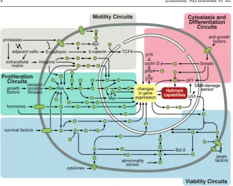
ii) viability circuits; iii) motility circuits; and iv) cytostasis and differentia-tion circuits (see Figure 1). The failure or dysreguladifferentia-tion of these four circuits jointly make up the characteristic phenotype of cancer cells, corresponding di-rectly with four of the hallmarks given above. In contrast to healthy cells that carefully control the production of specific growth and proliferative signals, cancer cells have an abnormal progression through the cell cycle and divide rapidly. Equally they have much higher viability compared to normal cells; resisting cell death, avoiding immune destruction, genome instability and mu-tation make cancer cells somewhat “immortal”. The outcome is the formation of macroscopic structures such as solid tumours that can be observed clinically. Despite enormous progress full understanding of these processes is difficult be-cause we are dealing with a complex interplay between various subprocesses occurring with different dynamics at different spatial scales.
One of the most dangerous properties of malignant tumours is their ability to invade surrounding tissues and to metastasize. The invasion or infiltration of surrounding tissue by cancer cells can impair the tissue or organ function. However, a more dangerous aspect of invasion is the infiltration of blood and lymph vessels. When cancer cells penetrate the vessel lumen they may migrate with blood or lymph to distant sites in the body to form new tumours, i.e. metastases. It is worth mentioning that angiogenesis also contributes; through the formation of new blood vessels within the tumour it facilitates the mi-gration of tumour cells. Metastasis of cancer makes patient’s treatment very difficult. It prevents the effective resection of the primary tumour, as new outbreaks cause recurrence of the disease. There are many mechanisms that enable cancer cells invasion and metastasis, together making the motility cir-cuit. One can mention here the frequently occurring over-expression of genes encoding extracellular matrix-degrading enzymes such as matrix metallopro-teinases (MMPs). However, perhaps the most characteristic change is the loss of the functionality of the protein E-cadherin, which is the main molecule responsible for binding between epithelial cells.
regu-Fig. 1 Key intracellular signalling pathways and the cell functions they are connected with, illustrating the connection between the intracellular scale and the cellular scale. Reprinted from Cell, 144(5), Hanahan, D., Weinberg, R.A., Hallmarks of Cancer: The Next Generation, 646-674, Copyright (2011), with permission from Elsevier.
lation and apoptosis, another important issue is how the disease progression is influenced by structural or epigenetic changes within the cell nucleus.
[image:4.595.72.411.71.341.2]Further milestones related to cancer modelling will be adapting the models for specific cancer types and specific patients. The latter means not only the acquisition of biochemical parameters but also the acquisition of medical image data for individual patients. This will be a definite step towards personalised medicine, which has a chance to completely reform our approach to the patient and his treatment. Already today imaging studies are of great importance in diagnosis and planning surgical procedures. However, especially for treatment of non-resectable tumours, such imaging studies could also be important in selecting the appropriate treatment or monitoring the disease dynamics.
In this paper we intend to promote two specific avenues of cancer modelling which consider processes at different scales. In Section 2 we discuss the mod-elling of intracellular dynamics, specifically gene regulatory networks (GRNs), using a spatial stochastic approach. Firstly we apply this approach to so-called synthetic GRNs: repressilators and explore the role of molecular movement in such systems. Secondly, we apply this approach to the NF-κB pathway, which is important in diseases such as cancer and the inflammatory response. In Sec-tion 3 we focus on the cell scale, in particular investigating cell-cell/cell-matrix dynamics using a force based model. Specifically we apply this to modelling avascular tumour chords around blood vessels. In Section 4 we remark on the importance of these two modelling approaches individually and discuss how coupling these techniques together to form a multi-scale framework offers a new horizon for cancer modelling. In particular using high performance com-puting (HPC) it would be possible to combine these two techniques whilst at the same time modelling 106−109 cells, thereby enabling one to model at the tissue scale.
2 Intracellular dynamics - GRNs
levels of the molecules involved. Furthermore, in many biological processes, it is the oscillatory expression which is of particular importance.
Mathematical modelling of GRNs began with the papers of Goodwin (1965) and Griffith (1968), in which a negative feedback model for a simple, sin-gle mRNA-protein feedback system was proposed. However, while GRNs are known to exhibit periodic fluctuations in mRNA and protein concentrations (e.g. the results for the Hes1 system, cf. Hirata et al. (2002)), these early models, which were restricted to purely temporal ODEs, could not derive os-cillatory behaviour. Since the late 1990s there has been interest in the study of delay-differential equation models for GRNs (e.g. Smolen et al., 1999, 2001, 2002; Tiana et al., 2002; Jensen et al., 2003; Lewis, 2003; Monk, 2003; Bernard et al., 2006), following on from Mackey and Glass (1977) who introduced the idea of incorporating delays into differential equations two decades years ear-lier. The inclusion of a delay in ODE models of GRNs (e.g. the Hes1 system, the p53-Mdm2 system and the NF-κB system) has been shown to produce the required oscillatory behaviour (e.g. Tiana et al., 2002; Jensen et al., 2003; Lewis, 2003; Monk, 2003; Bernard et al., 2006).
An alternate approach has been to model GRNs with reaction-diffusion PDEs rather than ODEs, to incorporate spatial aspects. The first such spatial models (for theoretical intracellular systems) were proposed in the 1970s by Glass and co-workers (Glass and Kauffman, 1970; Shymko and Glass, 1974) and similarly in the 1980s by Mahaffy and co-workers (Busenberg and Mahaffy, 1985; Mahaffy, 1988; Mahaffy and Pao, 1984). The inclusion of spatial terms rather than a delay equally leads to the necessary oscillations (e.g. Sturrock et al., 2011, 2012; Szyma´nska et al., 2014; Lachowicz et al., 2016; Macnamara and Chaplain, 2016). Furthermore, Chaplain et al. (2015) rigorously proved, for the Hes1 system, that molecular diffusion causes oscillations. It is worth noting that a few models incorporate both spatial aspects and delays (e.g. Momiji and Monk, 2008). At a time when biologists are developing techniques to tag and monitor the movement of molecules in single cells (e.g. Betzig et al., 2006; Manley et al., 2008; Spiller et al., 2010; van de Linde et al., 2011; Won et al., 2011; Bar-On et al., 2012; Hiersemenzel et al., 2013) it is important to have appropriate mathematical models that have the ability to analyse the spatial data that arises from such experiments.
The study of GRNs also plays both a theoretical and practical role in the field of synthetic biology. Since the pioneering work of Becskei and Serrano (2000) and Elowitz and Leibler (2000) onE. coli, there has been renewed in-terest in synthetic GRNs as a method of designing and constructing predictable biological systems (Balagadde et al., 2008; Chen et al., 2012; Yordanov et al., 2014) with concomitant studies of a more theoretical nature (Purcell et al., 2010; O’Brien et al., 2012; Macnamara and Chaplain, 2016). Such activities could in future lead to the development of better drug design, more efficient crop yields and enhanced bioenergy production (Yordanov et al., 2014).
to consider them stochastically. While GRNs are observed to exhibit peri-odic fluctuations (e.g. Hirata et al., 2002; Nelson et al., 2004; Geva-Zatorsky et al., 2006), results from intracellular imaging show inherent stochasticity (e.g. Spiller et al. (2010)). The noise may be caused by a combination of the underlying randomness of necessary events (such as the binding/unbinding of protein and promoter) and the natural variation of production and degra-dation rates (since transcription and translation occur in bursts rather than continually). Adding to that the fact that the molecular species involved are present in low numbers, continuum models are unlikely to provide an accurate description of the real life situation. Burrage and co-workers (e.g. Barrio et al., 2006; Tian et al., 2007; Marquez-Lago et al., 2010) were amongst the first to seek oscillatory behaviour of GRNs using a stochastic approach. They used a delay SSA method, SSA being the stochastic simulation algorithm developed by Gillespie (1976) and discussed how a time-delay could account for spatial aspects (Marquez-Lago et al., 2010), without the need to incorporate them explicitly. However, prompted to further investigate the importance of spatial aspects, Sturrock et al. (2013) designed a model of GRNs (specifically the Hes1 system) which accounts for the importance of both space and stochastic-ity. They used a continuous-time discrete-space Markov process to model the reaction-diffusion kinetics. Since cell populations are naturally heterogenous, a stochastic description with spatial aspects built in allows us to incorporate a variety of differences and to look for emergent behaviour. The approach of Sturrock et al. (2013) can be applied to model other natural pathways or synthetic GRNs and we give two such applications here.
At the heart of any model for GRNs lies a system of chemical/molecular reactions, which describe how different species interact. Within a continuum setting we are able to extrapolate from these a set of differential equations. A discrete approach by contrast relies on a chemical master equation; the spatial stochastic models we discuss here are continuous time, discrete space Markov processes governed by a reaction diffusion master equation (RDME). Model reactions (modelled with simple mass action kinetics) are localised at specific sites or regions within the cell. In the following section we give some selected results from the simulations of specific RDMEs (see Appendix A for more details of the basic model set-up).
2.1 GRN Simulation Results
Synthetic GRNs -n-gene repressilators
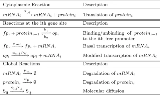
Table 1 List of the i-th molecular reactions in an n-gene repressilator system (adapted from the Hes1 system of Sturrock et al. (2013))
Cytoplasmic Reaction Description
mRN Ai αpi
−−→mRN Ai+proteini Translation ofproteini
Reactions at the ith gene site Description
f pi+proteini−1 b1
−−* )−−
b2 opi Binding/unbinding of proteini−1
to the ith free promoter
f pi αmi
−−−→f pi+mRN Ai Basal transcription ofmRN Ai
opi αmi/γi
−−−−−→opi+mRN Ai Modified transcription ofmRN Ai
Global Reactions Description
mRN Ai µm
−−→ ∅ Degradation ofmRN Ai
proteini µp
−−→ ∅ Degradation ofproteini
Sli
qlijxli
−−−−→Slj Molecular diffusion
Our model reactions are given in Table 1, fori={1,2, ...n}. Consider a genei, its mRNA is translated producing protein, within the cytoplasm, at a rateαpi. The (i−1)-th protein is then available to bind with (and then unbind from) its
i-th promoter at a specific gene site, with binding and unbinding ratesb1and
b2, respectively. Depending on whether the protein is bound with its promoter or not determines the rate of mRNA production for the following gene in the chain. A free (or unbound) promoter transcribes mRNA at the basal rateαmi,
while an occupied (or bound) promoter either enhances or diminishes mRNA production depending on the value ofγi. We assume that both species degrade
(at ratesµmandµp, respectively) and diffuse throughout the domain.
This single description may be used to model a variety of synthetic GRNs, with the nuances of each captured by changes to specific parameters. In partic-ular, we are able to model repression or activation of an mRNA by a preceding protein through changes to the parameterγi (Sturrock et al., 2013). Ifγi<1
the basal rate of mRNA transcription is enhanced when the preceding protein is bound to its promoter (there is positive feedback), whereas the basal rate of mRNA transcription is reduced when the preceding protein is bound to its promoter forγi >1 (there is negative feedback).
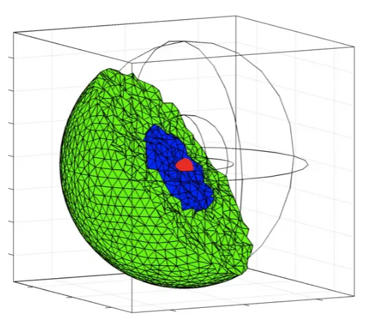
Fig. 2 Computational 3D cellular domain used in the stochastic spatial simulations con-sisting of a cytoplasm (green), a nucleus (blue) and gene binding sites within the nucleus (red). The nucleus has radius 3µm and the cell has radius 7.5µm. See text for full details.
Key to this modelling approach is the position of promoter sites, where the binding/unbinding and transcription reactions take place. How variations in the spatial location of the gene site (and also the protein production site) affect the levels of the molecules in GRNs has been explored in Sturrock et al. (2012); Macnamara and Chaplain (2016, 2017). This aspect remains to be explored more fully in a spatial stochastic setting. For our simulations of the three-gene repressilator, the three promoter sites are located at single voxels tightly clustered together within the nucleus. In Table 2 we give the parameter values used in the simulations.
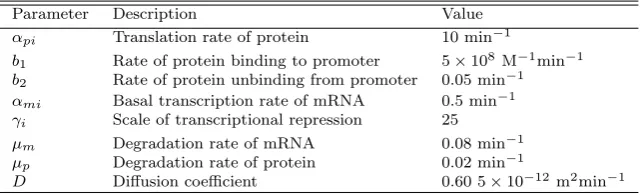
[image:9.595.105.386.84.314.2]Table 2 List of parameter values used in the computational simulations (all parameters are within ranges reported by Sturrock et al. (2013))
Parameter Description Value
αpi Translation rate of protein 10 min−1
b1 Rate of protein binding to promoter 5×10⁸ M−1min−1
b2 Rate of protein unbinding from promoter 0.05 min−1
αmi Basal transcription rate of mRNA 0.5 min−1
γi Scale of transcriptional repression 25
µm Degradation rate of mRNA 0.08 min−1
µp Degradation rate of protein 0.02 min−1
D Diffusion coefficient 0.60 5×10⁻¹²m2min−1
Natural GRNs - the NF-κB pathway
While a generic model of GRNs with simple feedback incorporated offers gen-eral insight into mRNA-protein dynamics, a spatial stochastic approach can easily be applied to more complex pathways which contain a variety of molec-ular interactions. Here we give a few selected simulation results for a spatial stochastic model of the NF-κB pathway, which when it works correctly is re-sponsible for coordinating processes such as adaptive and innate immunity, development and cell survival but if dysregulated may lead to chronic in-flammatory diseases, autoimmune diseases and the initiation and progression of cancer. Nuclear factor κB (NF-κB) was discovered in 1986 as a nuclear factor in B lymphocytes responsible for regulating the gene encoding the im-munoglobulinκlight polypeptide chain. It is found to be present in almost all mammalian cell types and is activated in response to many different stimuli, including environmental cues such as hypoxia and ultraviolet radiation; infec-tious agents, such as bacteria and viruses; and extra- and intracellular stress, such as inflammatory cytokines and DNA damage. Due to the diversity of the means to NF-κB activation, it is not surprising that NF-κB has been found to have the potential to control the transcriptional activity of over three hundred genes and to thus play a role in many different processes.
to the nucleus, binding to nuclear NF-κB and transporting it back to the cyto-plasm (Arenzana-Seisdedos et al., 1997). Particular examples of extracellular stimuli that activate the canonical NF-κB signalling pathway are the pro-inflammatory cytokine, tumour necrosis factor α (TNFα), and the bacterial product, lipopolysaccharide (LPS). Upon ligand binding to a specific cellular membrane receptor, such as tumour necrosis factor α receptor 1 (TNFR1) or Toll like receptor 4 (TLR4), adaptor molecules, kinases and ubiquitin lig-ases are recruited, leading to the activation of the TAK–TAB complex (TGF [transforming growth factor]β activated kinase–TAK associated binding pro-tein). TAK is essential for the activation of the trimeric complex, IKK (the inhibitor of IκB kinase), which in mammalian cells is composed by IKKα, IKKβand IKKγ. IKK activation leads to phosphorylation of the IκBαwithin an IκB/NF-κB complex at amino acid residue serine 32 and serine 36. This phosphorylation of IκB is a marker for it to be tagged for ubiquitination. Once ubiquitinated it is degraded by the proteasome, thus releasing NF-κB to translocate to the nucleus, where it binds toκB sites in the promoters and en-hancers of its target genes. The full set of reactions/interactions for the NF-κB pathway are given in Tables 6-8 in Appendix B.
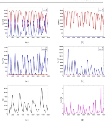
Here we give simulation results of the RDME for the NF-κB pathway. A single realisation of the experiment is shown in Figure 5. Again, in this case the computational domain consists of two concentric spheres (the outer sphere representing the cytoplasm - radius 9.5µm - and the inner sphere representing the nucleus - radius 5µm) and three individual gene/promoter sites for NF-κB, IκB and A20 localised within the nucleus (specifically, the NF-κB gene site is located at the origin, and the IκB and A20 gene sites have displacements of 2.5µm and −2.5µm respectively along thex Cartesian axis from the origin). The plots given in Figure 5 show periodic fluctuations in the copy numbers of NF-κB, IκB (and the complex of the two) along with A20 as well as indicating periodicity in the NF-κB cytoplasmic ratio which suggests nuclear-cytoplasmic oscillations.
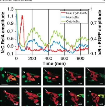
Fig. 4 Top panel: temporal oscillations of key molecular species in the NF-κB system. Bottom panel: experimental observation of spatio-temporal oscillations in NF-κB localisa-tion in individual cells. This figure shows time-lapse confocal images of NF-κB-containing species fused to a red fluorescent protein and of IκBa-containing species fused to a green fluorescent protein in SK-N-AS cells after stimulation with TNFa. The arrow marks one oscillating cell. Nuclear-cytoplasmic translocation of NF-κB-containing species is apparent. Time is shown in minutes and the scale bar represents 50µm. From Nelson, D. E., Ihekwaba, A. E. C., Elliott, M., Johnson, J. R., Gibney, C. A., Foreman, B. E., Nelson, G., See, V., Horton, C. A., Spiller, D. G., Edwards, S. W., McDowell, H. P., Unitt, J. F., Sullivan, E., Grimley, R., Benson, N., Broomhead, D., Kell, D. B., White, M. R. H., 2004. Oscillations in NF-κB signaling control the dynamics of gene expression. Science 306, 704-708. Reprinted with permission from AAAS.
[image:13.595.72.412.72.416.2](a) (b)
(c) (d)
(e) (f)
Fig. 5 Plots showing temporal oscillations of key molecular species in the NF-κB system obtained from simulations of the spatial stochastic model. From top left to bottom left: time series (spanning 1600 minutes) for the copy number of (a) total NF-κB (b) total IκB–NF-κB complex, (c) free NF-κB, (d) free IκB, (e) total A20, respectively. In the bottom right plot, (f), we give the NF-κB nuclear-cytoplasmic ratio. Where applicable (in figures (1)-(d)) the total number of cytoplasmic species is indicated in red and the total number of nuclear species is indicated in blue. Parameter values given in Appendix B in Tables 6-8.
3 A Multiscale Individual-based Model of Cancer Growth
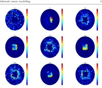
[image:14.595.75.418.73.468.2]Fig. 6 Plots of the spatial distribution of NF-κB molecules inside a cell at times t=0, 42, 84, 128, 196, 292, 356, 400, 464 minutes. Cross-section through the middle of the cell from the full 3D simulation. Parameter values given in Appendix B in Tables 6-8.
cell level. There are now a number of different individual-based modelling ap-proaches that one can adopt cf. cellular automata, Cellular Potts Model, hybrid discrete-continuum (Anderson and Chaplain, 1998; Alarcon et al., 2003; An-dasari et al., 2012; D’Antonio et al., 2013). Here we adopt an individual-based, force-based model of cell growth which is driven by forces acting upon the cell, and is based upon the model of Ramis-Conde et al. (2008). More recently this approach has been extended and implemented on a massively parallel system (IBM Blue Gene/Q system) allowing hybrid high performance simulations to describe, for example, tumour growth in its early clinical stage. Details of the implementation can be found in Cytowski and Szyma´nska (2014, 2015b,a). Adopting this approach, we model each cell as an isotropic elastic object ca-pable of migration and division and parameterise it by cell-kinetic, biophysical and cell-biological parameters that can be experimentally measured, from both
[image:15.595.78.406.67.350.2]0 10 20 30 40 50 60 70 80 90 100 0
50 100 150 200
mean period
cell index
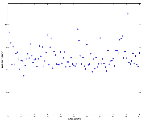
Fig. 7 Plot showing the mean period (in minutes) of total NF-κB for 100 simulations of the spatial stochastic model. The periods were calculated using a Morlet continuous wavelet transform with Gaussian edge elimination. Parameter values given in Appendix B in Tables 6-8.
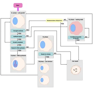
Regarding cell kinetics, we assume that the cell-cycle is divided into four phases, i.e. mitosis - M-phase, followed by G1-, S-, and G2-phases, after which mitosis occurs again. During a complete cell-cycle, the cell must accurately duplicate its DNA once during S-phase and distribute an identical set of chro-mosomes equally to two progeny cells during M-phase. M-phase consists of two major events: the division of the nucleus called mitosis and subsequent cytoplasmic division called cytokinesis. G1-phase is an interval between mito-sis and the initiation of nuclear DNA replication. It provides additional time for a cell to grow and to replicate its cytoplasmic organelles. G2-phase is again an interval between the completion of nuclear DNA replication and mitosis. Over the course of both the G1- and G2-phases, the cell checks the internal and external environment to ensure that the conditions are suitable and complete preparation for entry into either S-phase or M-phase. When DNA is damaged cell cycle is arrested in G1 or G2 so that the cell can repair DNA damages prior to its duplication or before cell division.
[image:16.595.100.381.103.345.2]Fig. 8 Schematic diagram showing the cell cycle and cell dependency upon availability of nutrients used in the individual-based model.
that cell division cannot start before DNA replication is complete. Similarly, when DNA is damaged the cell cycle is arrested so that the cell can repair the damage. This is possible because the cell is equipped with molecular mecha-nisms that can stop the cycle at various checkpoints. Two main checkpoints are located within the G1- and G2-phases. The G1 checkpoint allows the cell to check whether its environment is conducive to divisions and whether its DNA is damaged. If environmental conditions make cell division impossible, instead of entering S-phase a cell can enter a resting state - G0-phase, where it remains until conditions improve and it continues the cell cycle. The G2 check-point ensures that the cell has no DNA damage, and DNA replication will be completed before the beginning of mitosis (Alberts et al., 2010). A simplified schematic of the cell-cycle model and cell interactions with the environment used in our computational simulations is given in Figure 8.
[image:17.595.80.408.87.400.2]distancedcicj between the centres of two adjacent cells,ci andcj, of radii,rci
andrcj, both their surface contact area and the number of adhesive contacts increase, resulting in an attractive interaction. We assume that adhesive forces are proportional toρm, which is the density of the surface adhesion molecules in the contact zone (which we assume is given for particular cell type), kB,
which is the Boltzmann constant, T, which denotes temperature and Dcicj,
which measures the contact between cells ci and cj and is calculated as the
volume of the common area of intersecting spheres representing those cells. Experiments suggest that cells only have a small compressibility - the Poisson numbers are close to 0.5, (Mahaffy et al., 2000; Alcaraz et al., 2003). In this instance, both the limited deformability and the limited compressibility give rise to a repulsive interaction. Repulsive forces are inversely proportional to the term Eci,cj, which is calculated form Young moduli, Eci and Ecj, and
Poisson ratios,νci andνcj. The precise formula is given by:
Eci,cj =
3 4
1−νc2 i
Eci +
1−ν2
cj
Ecj
(1)
We model the combination of the repulsive and attractive energy contributions by a modified Hertz-model (Galle et al., 2005; Schaller and Meyer-Hermann, 2005) which has the advantage that both the interaction energy and the force can be represented as an analytical expression (Drasdo and H¨ohme, 2005). Inertia terms are neglected due to the high friction of cells with their envi-ronment, and we also do not consider the existence of any memory term as in Galle et al. (2005).
Vcicj = (rci+rcj−dcicj) 5
2 1
5Ecicj
r r
circj
rci+rcj
| {z }
repulsive interactions
+ρmDcicj25kBT
| {z }
adhesion
(2)
Cells require access to oxygen from the circulatory system in order to grow and survive. It is well known that cancer cells grow preferentially around blood vessels. Those tumour cells that are located more than about 0.2 mm away from blood vessels were found to be quiescent, while others even farther away were found to be necrotic. This threshold of approximately 0.2 mm represents the distance that oxygen can effectively diffuse through living tissue (Weinberg, 2007). Because of the low redox potential and high activation energy that occurs in living organisms, reactions involving molecular oxygen occur only in mitochondria. Therefore, we assume that the loss of oxygen in the tissue takes place only due to its consumption by the cells. The general equation governing the external oxygen concentrationQ(x, t) in the cells’ environment may be written:
∂
∂tQ(x, t) =DQ∇
of oxygen by vessels. Both of these functions are computed in each time step of the simulation from the current spatial organisation of cells and vessels through interpolation. The force associated with a given cell,ci, is then given by the expression:
Fci= ∇Vci
| {z } inter-cellular interactions
+λ∇Q(x, t)
| {z }
chemotaxis
(4)
whereλis a measure of a cell’s chemotactic sensitivity to the oxygen concen-tration andVci is given by
Vci= X
cj∈Bci(ci)
Vcicj (5)
with Bci(ci) a sphere (i.e. a ball inR3) centred on (xci, yci, zci), radiusci,
denoting the maximum inter-cellular interaction region.
Summing all the forces between the cells and assuming a frictional force/drag force proportional to a cell’s velocity and then applying Newton’s Second Law of motion allows us to integrate a Langevin-type equation to give the spatial location of the cells over time. The direct use of equations of motion for the cells permits one to include more easily the limiting case of very small (or no) noise and is more intuitive. In this approach cells move under the influence of forces and a random contribution to the locomotion which results from the local exploration of space.
Solving the oxygen concentration (which is a global field) together with the individual-based particle system of up to 109 cells is a challenging task in the context of parallel processing. First of all, it requires the use of appropriate data structures to optimize the computations of interactions between lattice-free cells. In our approach, the main data structure that stores information about cells is an octal tree. We assume that the domain of simulation is a 3D cube. The cells are arranged in a tree based on the position of their centers. The tree is built recursively starting from the whole domain of simulation, which corresponds to the root of the tree. Subsequently, the cubes are divided recursively into 8 equal cubes with edges reduced by a factor of a half. This procedure is repeated until in the cube under consideration there is only one cell centre.
Fig. 9 A 2D example of domain decomposition assigning cells to different processors. Local cells of each process are denoted by the same colour. Our aim was to minimize the execution time and enable good parallel scalability on massively parallel systems. Our decomposition algorithm is based on Peano-Hilbert space filling curves. Such a method ensures the property of geometrical locality which is very important when computing cell-cell interactions in a given neighbourhood.
load-balancing method (e.g. geometrical load-balancing method) has the very nice property of geometrical locality which is very important when computing cell-cell interactions in a given neighbourhood, see Figure 9.
The equation governing the external oxygen concentration is equipped with Dirichlet boundary conditions and is discretised with an implicit in time finite difference scheme. The resulting linear system is then defined in the ParCSR parallel format and solved with the Conjugate Gradient method precondi-tioned by the BoomerAMG algebraic multigrid method (both available in the Hypre library, cf. Baker et al. (2012)). The domain decomposition scheme used for the finite-difference numerical scheme is different from the one used for a particle system. For data modelled in a continuous manner the data decom-position is achieved by assigning 3D grid blocks to different processes.
[image:20.595.165.315.94.257.2]Scheme 1Pseudo-code outlining the algorithm followed in the HPC simula-tion of the individual-based model
iter←0
whileiter≤max iterdo
Step 1: Perform domain decomposition; Step 2: Build tree;
Step 3a: Find exchange regions and initiate data exchange;
for alllocal cellsdo
Step 4a: Find cell’s neighbours←local data;
Step 5a: Compute potential and density functions←local data;
end for
Step 3b: Wait until data exchange is finished;
for alllocal cellsdo
Step 4b: Find cell’s neighbours←remote data;
Step 5b: Compute potential and density functions←remote data;
end for
Step 6: Interpolate cells to global fields grid; Step 7: Compute global fields;
Step 8: Interpolate global fields to cells;
for alllocal cellsdo
Step 9: Update cells’ cycle;
Step 10: Compute forces and move cells to their new positions;
end for
iter ++;
end while
3.1 Application to tumour cords
Fig. 10 Tumour cells surrounding a central blood vessel from a Dunning rat prostate carcinoma xenograft Hlatky et al. (2002). Regions of viable tumour cells (cuffs) are formed around the central vessel. The dashed black line indicates the boundary of the region. Cuff size is roughly indicative of the metabolic burden of the carcinoma cells. Tumour cells within approximately 110µm of the vasculature are viable. Beyond this zone oxygen and nutrient levels drop below a critical threshold and an area of necrosis is observed. From Hlatky, L., Hahnfeldt, P., Folkman, J., Clinical application of anti-angiogenic therapy: microvessel density, what it does and doesnt tell us. J. Natl. Canc. Inst. 2002, 94(12), 883-893, by permission of Oxford University Press.
Parameter estimation
parameters used in the individual-based model is given in Table 3.
Table 3 Description of the parameters used in the individual-based model and their values along with the relevant reference.
Description Value Reference
Average cell diameter (EMT6 tumour cell line)
10µm Casciari et al. (1992) G1 phase length (EMT6
tu-mour cell line)
11h Zacharaki et al. (2004) S phase length (EMT6 tumour
cell line)
8h Zacharaki et al. (2004) G2 phase length (EMT6
tu-mour cell line)
4h Zacharaki et al. (2004) M phase length (EMT6
tu-mour cell line)
1h Zacharaki et al. (2004) Oxygen diffusion coefficient in
multicellular spheroids
[1.65−1.9]×10−5cm2s−1 Mueller-Klieser and
Sutherland (1984) Oxygen consumption rate of
proliferating cells (EMT6 tu-mour cell line)
16.9 × 10⁻¹⁷mol s−1
cell−1
Walenta and Mueller-Klieser (1987)
Oxygen consumption rate of quiescent cells (EMT6 tumour cell line)
9.6×10⁻¹⁷mol s−1cell−1 Walenta and
Mueller-Klieser (1987)
3.2 Computational simulation results
In Figures 11 and 12 we show computational simulation results for a tumour cord growing around a blood vessel for the baseline parameter case, as detailed in Table 3. Specifically the simulation is of an avascular cancer; the cancer cells are initiated around a central small blood vessel which secretes oxygen. The oxygen concentration is held constant on the vessel boundary and then diffuses to zero over a distance of around 200µm. We observe that as the mass of tumour cells grows, cells become hypoxic and then subsequently necrotic at which point they are coloured black. The numbers of viable and necrotic cells at various times from the computational simulation are given in Table 4. This mirrors the experimental findings of Hlatky et al. (2002), see Figure 10.
Table 4 Numbers of viable and necrotic cells at various times from the computational simulation shown in Figures 11 and 12.
Time (hours) # viable cancer cells # necrotic cells
332 739 54
443 1287 377
776 2443 2204
1332 3801 6478
Fig. 11 Plot showing the growing tumour cord around a central blood vessel at times 332, 443, 776 and 1332 hours. As the tumour cord grows, cells further away from the vessel become necrotic (black). At the final time of 1332 hours, there is a total of 10279 cells comprising 3801 viable cancer cells and 6478 necrotic cells. See text for details.
around the central vessel. The numbers of viable and necrotic cells at various times from the computational simulation are given in Table 5.
Fig. 12 Plot showing cross-sections of the growing tumour cord around a central blood vessel at times 332, 443, 776 and 1332 hours.. As the tumour cord grows, cells further away from the vessel become necrotic (black). At the final time of 1332 hours, there is a total of 10279 cells comprising 3801 viable cancer cells and 6478 necrotic cells. See text for details.
Table 5 Numbers of viable and necrotic cells at various times from the computational simulation shown in Figures 13 and 14.
Time (hours) # viable cancer cells # necrotic cells
332 815 1
443 2033 67
776 5469 1569
1332 9271 7452
multiple vessels. This more closely aligns with a realistic tissue environment which is perfused with many capillaries in close proximity with each other.
Fig. 14 Plot showing cross-sections of the growing tumour cord around a central blood vessel under reduced oxygen consumption at times 332, 443, 776 and 1332 hours. As the tumour cord grows, cells further away from the vessel become necrotic (black). At the final time of 1332 hours, there is a total of 16723 cells comprising 9271 viable cancer cells and 7452 necrotic cells. See text for details.
4 Discussion and Conclusions
As noted in the Introduction, the development of cancer is a true multiscale process connecting many scales through time and across space (cf. Hanahan and Weinberg (2000, 2011)). In this paper, we have presented models for as-pects of cancer growth at two of the “fundamental scales”; the intracellular level and the cellular level.
(a) (b)
[image:28.595.74.432.71.434.2](c) (d)
Fig. 15 Plots showing the computational simulation results of a tumour cord interacting with two blood vessels. Top Row: (a) Tumour cord growing around two vessels. (b) Tumour cord growing around two vessels later time. Bottom Row: (c) Oxygen profile levels in the tumour cord. (d) Cross section showing corresponding development of tumour cells.
one based at the cell level, as we discuss next, would further strengthen our understanding of cancer dynamics.
In Section 3 we discussed a multi-scale computational framework which focussed on the cell scale. At the heart of the framework is an individual-based, force-based model of cancer cell growth. The model was originally de-veloped by Ramis-Conde et al. (2008) who in turn dede-veloped earlier work by Drasdo and H¨ohme (2005). By taking advantage of recent developments in high-performance computing techniques, we have carried out our simulations of the model on a massively parallel computer. This has enabled us to simu-late up to the level of tens of thousands of cells in an acceptable timeframe. We have shown some simple proof of concept simulations to show how the model can replicate solid tumour growth. In particular we have considered the proliferation of cancer cells around blood vessels - so called tumour cords.
The use of HPC will allow our computational framework for the individual-based model to reach the tissue scale (109 individual, interacting cells which translates into a volume of approximately 1cm3, i.e. a sizeable volume at the tissue scale) and as such it can be used to simulate tissue-level phenomena. The feasibility of such an approach in terms of computational time has been explored by Cytowski et al. (2017) where the growth of a solid tumour de-veloping in healthy tissue was simulated. A single tumour cell was placed in the centre of an initial mass of 194,100,035 (≈ 1.9×10⁸) healthy cells and allowed to grow in response to an external oxygen field. The final tissue configuration consisted of 245,890,017 healthy cells (≈2.5×10⁸) and 73,836 cancer cells, with the simulation taking a single day using 128 cores of the IBM Power 775 system Cytowski et al. (2017). The results of this study con-cluded that a single time step of the simulation, corresponding to 1 hour in real time, took 100s of computational time. Therefore, for example, to sim-ulate a (real time) three-month growth period of a solid tumour would take 100s×(24h×30days×3) = 216000s = 60hours = 2.5days.
for in the model implicitly through the external frictional/drag force). This could be done in several ways - model the tissue/stroma as a different cell type (Cytowski et al., 2017), model the tissue/stroma as a collection of individual fibres (Schl¨uter et al., 2015), model the tissue/stroma as another cell type and a collection of individual fibres, model the tissue/stroma as another external field satisfying a PDE similar to the external oxygen (Jagiella et al., 2016). Any one of these approaches would be more akin to modelling the cells mov-ing through a porous medium. The approaches of Cytowski et al. (2017) and Jagiella et al. (2016) would have minimal increase in computational time but the approach of Schl¨uter et al. (2015) is computationally more expensive. The computational cost of simulating large numbers of cells interacting with indi-vidual fibres in 3D would have to be explored, although initial estimates in 2D for small numbers of cells can be found in Schl¨uter et al. (2015). Incorporating intracellular signalling pathways into the multi-scale model will also increase the computational simulation time. Indeed, embedding a system of stochastic PDEs within each cancer cell would be computationally prohibitive. However, it is also not necessary since many of the key gene regulatory networks associ-ated with cancer (e.g. p53-Mdm2, NF-κB) are not operative continually, but begin to function and upregulate the molecules when there is some external stimulus - in the case of p53, when DNA damage occurs or a cell experi-ences hypoxia. The oscillations in the levels of the molecules in such systems are normally on the order of a few hours which is shorter than the growth timescale of a solid tumour. One approach which would be computationally feasible would be to exploit the difference in timescales i.e. stop the growth of the cancer cells when an external stimulus was applied, carry out simulations of the intracellular GRNs modelling a period of several hours at which point the effect of the GRNs at a cell/phenotypic level could be determined. Key cell-level parameters connected to the activity of the GRNs, e.g. cell cycle ar-rest, cell proliferation rate, apoptosis, could then be modified in a number of the cancer cells. Modelling the intracellular activity would then be halted and the modelling of the growth of the cells would then continue. A similar com-putational strategy has been successfully adopted by (McDougall et al., 2006) in modelling the growth of blood vessel networks - the different time-scales between blood flow dynamics and endothelial cell growth have been exploited to model a so-called dynamic-adaptive blood vessel network.
software developed at the Interdisciplinary Centre for Mathematical and Com-putational Modelling (ICM, Warsaw), allowing complex visual analysis and segmentation of the geometry to be studied. On the basis of the chosen geom-etry we can develop digitised input data for our computational model. Figure 16 shows an example of a blood vessel geometry imported from heart microto-mography. First, the relevant clinical/medical structures are segmented. Then, on the basis of the geometry obtained, again applying the VisNow package, we create a mesh that after some smoothing and filtering procedures is used as the input for the generation of the actual initial data. At each point of the mesh we locate a cell. The final step consists of removing unnecessary cells i.e. those that are too close to others. As imagining techniques develop fur-ther, they will be able to provide even finer detail, higher resolution and image smaller structures, and it should be possible to create “computational capil-laries” at the correct spatial scale around which cancer is initiated. The model of solid tumour growth and interaction with blood vessels can also be further developed to explicitly include blood flow through the vessels and the impact that flow has on the vessel network structure through dynamic adaptation (cf. McDougall et al. (2006); Macklin et al. (2009)). This in turn could lead to a multiscale model of chemotherapy treatment of cancer. In more general terms, the modelling approach can be applied to many other important pro-cesses such as wound healing, embryogenesis, tissue engineering and cardiac tissue modelling where tissue level phenomena depend upon, and also in turn influence, interactions and phenomena at both the cell and intracellular levels.
Finally, given the timing of this special issue, it is perhaps apposite to end with a quotation from Professor Sir D’Arcy Wentworth Thompson, whose seminal book “On Growth and Form” was published exactly one century ago:
“...numerical precision is the very soul of science, and its attainment af-fords the best, perhaps the only criterion of the truth of theories and the cor-rectness of experiments ...I know that in the study of material things number, order, and position are the threefold clue to exact knowledge: and that these three, in the mathematician’s hands, furnish the first outlines for a sketch of the Universe.” (Thompson, 1917).
While “sketching the universe” is on yet another completely different scale, the essence of the above quotation, that mathematical modelling can provide quantitative insight to biomedical systems, is still relevant and even more timely today. Echoing the words of D’Arcy Thompson, one century on, we may say that computational multiscale mathematical modelling furnishes not only the first outlines for a sketch of cancer growth but provides the basis for the development of a virtual solid tumour. Cura ex macchina – in silico
Appendices
A The Reaction-Diffusion Master Equation
Here we described in the set-up for the spatial stochastic model for intracellular GRN dy-namics. We describe the computational domain and how reaction and diffusion events are incorporated into the reaction diffusion master equation (RDME). We also provide some notes on how simulations are produced. For a more detailed description see the supplemen-tary material of Sturrock et al. (2013).
A.1 The Computational Domain
The computational domain (see Figure 2, for example) is set-up using COMSOL and a mesh is imposed. In general the domainΩis meshed intoV tetrahedra shaped subvolumes, voxels,
Ωk, k∈ {1, .., V}such that,
Ω=
V [
k=1
Ωk, and Ωi∩Ωj=∅,∀i6=j, i, j∈ {1, .., V}.
At any given time the state of the system is described by the number of each chemical species within the domain. Changes to the state will either be by the chemical reactions at the voxel level or the movement (diffusion jumps) of a molecule between neighbouring voxels.
A.2 Chemical Reactions
We consider reactions that occur due to molecular contact. We assume that the species of our system, within each subvolume, are uniformly distributed and in thermal equilibrium, such that the motion of each molecule is random. We consider the probability of a collision occurring between two reactant molecules. The likelihood of a reaction occurring, changing the state of the system fromxtox+Nr is determined by its reaction rate, described by
the reaction propensity functionωr(x). As such reactions can be described by
x−−−−→ωr(x) x + Nr,
whereNr∈ZSis the transition step, defined by therth column of the stoichiometric matrix
M andωr(x) is the probability that the reaction occurs during a infinitesimal time interval,
i.e.
ωr(x) = lim dt→0
P(x+Nr, t+dt)−P(x, t)
dt
A.3 Molecular Diffusion
The movement of a chemical speciesSl from a voxelψi to a randomly selected adjacent
voxelψjdescribes the molecular diffusion and is modelled as a first-order event. As such we
treat the diffusive process in a similar way to a reactive process and consider the probability of a transition taking place i.e. the probability for one of thelthspecies to make a jump from theithsubvolume to an adjacentjthsubvolume. Hence, we consider the following,
Sli
qlijxli
where xli is number of speciesl located in voxeli andqlij is the diffusion rate constant
which depends on the macroscopic diffusion coefficient of speciesl(Dl) and the mesh of the
domain, specifically the shape and size of voxelsψiandψj. Note eachqlijis only non zero
for connected mesh elements and of the types of species we model only mRNAs and proteins diffuse, the free and occupied promoters remain permanently within the voxel assigned as the promoter site.
A.4 Solving the System
The temporal evolution of the probability distribution of each state in the statespace is governed by the reaction diffusion master equation (RDME). We complete the model set-up with zero-flux boundary conditions at the cell membrane, while we impose continuity of flux on the nuclear membrane. For initialisation we suppose that there is only a single free promoter within each promoter site. All simulations found in this paper are produced using the URDME (Unstructured Reaction Diffusion Master Equation) software framework (Drawert et al., 2012), which implements the next subvolume method (NSM) (Gibson and Bruck, 2000); the NSM being far more computationally efficient than the classical SSA for a 3D domain such as ours. URDME uses unstructured tetrahedral and triangular meshes (such as shown in Figure 2) for which diffusion rate constantsqlij are automatically computed
(Engblom et al., 2009; Drawert et al., 2012).
B NF-κB Reactions
Table 6 Cytoplasmic reactions
Cytoplasmic Reaction Description Parameter value Stimulus−−→α IKKa Activation of IKKa via
interaction with stimu-lus
α= 0.0015M min−1
IKKa + IκBNF−κB−−→A1 IKKaIκBNF−κB Formation of IKKa and IκBNF-κB complex
A1= 9×10¹⁰M−1min−1
IKKaIκBNF−κB−−→C1 IKKa + NF−κB Catalytic degrada-tion of IκB in the IKKaIκBNF-κB com-plex
C1= 1M−1min−1
IκBtran−−→SI IκBtran + IκB Translation of IκB pro-tein
SI= 1.5min−1
A20tran −−→SA A20tran + A20 Translation of A20
pro-tein
SA= 1.25min−1
A20 + IKKa−−→AD A20 + IKKn Deactivation of IKKa via interaction with A20
AD= 7×10⁸M−1min−1
IKKa−−→dk IKKn Spontaneous deactiva-tion of IKKa
dk= 0.055min−1
A20−−→ ∅dp Degradation of A20 dp= 0.07min−1
NF−κBtran−−→SN NF−κBtran + NF−κB NF-κB synthesis SN= 1min−1
NF−κB−)−−−−N−−−−−σon*
Nσof f
NF−κBmic NF-κB bind-ing/unbinding to microtubule
Nσon= 1×10⁹min−1
Nσof f = 10min−1
IκB−−−−)I−−−−σon*
Iσof f
IκBmic Binding/unbinding of IκB to microtubule
Iσon= 1×10⁹M−1min−1
Iσof f = 10min−1
N σi−−→v N σj Radially directed
ac-tive transport of
NF-κB between connected voxels
v= 3×10⁻⁵m min−1
Iσi−−→v Iσj Radially directed
ac-tive transport of IκB between connected voxels
v= 3×10⁻⁵m min−1
Sij
djik
Table 7 Reactions at gene sites
IκB gene site reactions Description Parameter value IκBpf+ NF−κB
b1
−−* )−−
b2 IκBpo Binding/unbinding of
NF-κB to the free IκB pro-moter
b1= 1×10⁸M−1 min−1
b2= 0.1min−1
IκBpo αI
−−→IκBpo+ IκBtran Induced transcription of
IκB mRNA
αI= 2.1min−1
IκBpf αI/γ
−−−−→Ipf+ IκBtran Basal transcription of IκB
mRNA
αI= 2.1min−1, γ= 80
IκB + IκBpo
binI
−−−→IpoI IκB binding to NF-κB oc-cupied IκB promoter
binI= 1×10⁹M−1 min−1
IpoI−−−→catI IκB + IκBp
f IκB induced NF-κB
degra-dation from Iκpromoter
catI= 1×10⁹M−1min−1
IpoI−−→sqI IκBNF−κB + IκBpf IκB sequesters NF-κB
from Iκpromoter
sqI= 1×10⁹M−1min−1
NF-κB gene site reaction Description Parameter value NF−κBpf
αN/γ
−−−−→NF−κBtran NF-κB mRNA transcrip-tion
αN= 0.5min−1, γ= 80
A20 gene site reactions Description Parameter value
A20pf+ NF−κB
k1
−−* )−−
k2 A20po Binding/unbinding of
NF-κB to the free A20 pro-moter
k1= 1×10⁸M−1min−1
k2= 0.1min−1
A20po αA
−−→Apo+A20tran Induced transcription of
A20 mRNA
αA= 2min−1
A20pf αA/γ
−−−−→A20pf+A20tran Basal transcription of A20
mRNA
αA= 2min−1, γ= 80
IκB +A20po
P
−−→IpoA IκB binding to the NF-κB occupied A20 promoter
P = 1×10⁹M−1min−1
IpoA−−−→catA IκB +A20p
f IκB induced NF-κB
degra-dation from Iκpromoter
catA= 1×10⁹M−1min−1
IpoA−sq−−A→IκBNF−κB +A20pf IκB sequesters NF-κB
fromA20 promoter
Table 8 Global reactions
Global Reactions Description Parameter value IκB + NF−κB−−→A2 IκBNF−κB Formation of IκB and
NF-κB complex
A2= 9×10¹¹M−1min−1
IκBNF−κB−−−→IDC NF−κB Natural degradation of IκB within IκBNF-κB
IDC= 0.000055min−1
IκBNF−κB−−−→NDC IκB Natural degradation of NF-κB within Iκ
BNF-κB
N DC= 0.000025min−1
IκBtran−−→ ∅dm Degradation of IκBtran
dm= 0.02min−1
IκB−−→ ∅dp Degradation of IκB dp= 0.07min−1
A20tran −−→ ∅dm Degradation of
A20tran
dm= 0.02min−1
Nuclear reactions Description Parameter value used Sij−−−→djik Sik Molecular diffusion of
species not containing IKKa
Acknowledgements ZS acknowledges the support of the National Science Centre Poland Grant 2011/01/D/ST1/04133, National Science Centre Poland Grant 2014/15/B/ST6/05082 and The National Centre for Research and Development Grant
STRATEGMED1/233224/10/NCBR/2014. MAJC and CKM gratefully acknowledge sup-port of EPSRC grant no. EP/N014642/1 (EPSRC Centre for Multiscale Soft Tissue Me-chanics – With Application to Heart & Cancer). EM was supported by an EASTBIO PhD Fellowship. The authors thank Bartosz Borucki from ICM for his help in with theVisNow medical imaging software.
References
Alarcon, T., Byrne, H., Maini, P., 2003. A cellular automaton model for tumour growth in inhomogeneous environment. J. Theor. Biol. 225, 257–274. Alberts, B., Bray, D., Hopkin, K., Johnson, A., Lewis, J., Raff, M., Roberts,
K., Walter, P. (Eds.), 2010. Essential Cell Biology. Garland Publishing, Inc., New York & London.
Alcaraz, J. L., Buscemi, M., Grabulosa, X., Trepat, B., Fabry, R., Farre, D., Navajas, D., 2003. Microrheology of Human Lung Epithelial Cells Measured by Atomic Force. Biophys. J. 84, 2071–2079.
Andasari, V., Roper, R., Swat, M. H., Chaplain, M. A. J., 2012. Integrating intracellular dynamics using CompuCell3D and Bionetsolver: Applications to multiscale modelling of cancer cell growth and invasion. PLoS ONE 7(3), e33726.
Anderson, A. R. A., Chaplain, M. A. J., 1998. Continuous and discrete math-ematical models of tumour-induced angiogenesis. Bull. Math. Biol. 60, 857– 899.
Arenzana-Seisdedos, F., Turpin, P., Rodriguez, M., Thomas, D., Hay, R. T., Virelizier, J. L., Dargemont, C., 1997. Nuclear localization of IκB alpha promotes active transport of NF-κB from the nucleus to the cytoplasm. J. Cell Sci. 110 (Pt 3), 369–378.
Ashall, L., Horton, C. A., Nelson, D. E., Paszek, P., Harper, C. V., Sillitoe, K., Ryan, S., Spiller, D. G., Unitt, J. F., Broomhead, D. S., Kell, D. B., Rand, D. A., S´ee, V., White, M. R. H., 2009. Pulsatile stimulation determines timing and specificity of NF-κB - dependent transcription. Science 324, 242– 246.
Baker, A. H., Falgout, R. D., Kolev, T. V., Yang, U. M., 2012. Scaling hypre’s multigrid solvers to 100,000 cores. In: Berry, M. W., Gallivan, K. A., Gal-lopoulos, E., Grama, A., Philippe, B., Saad, Y., Saied, F. (Eds.), High-Performance Scientific Computing. Springer, pp. 261–279.
Balagadde, F. K., Song, H., Ozaki, J., Collins, C. H., Barnet, M., Arnold, F. H., Quake, S. R., You, L., 2008. A synthetic escherichia coli predator– prey ecosystem. Mol. Syst. Biol. 4:187.
Barrio, M., Burrage, K., Leier, A., Tian, T., Sep 2006. Oscillatory regulation of hes1: Discrete stochastic delay modelling and simulation. PLoS Comput. Biol. 2 (9), e117.
Becskei, A., Serrano, L., 2000. Engineering stability in gene networks by au-toregulation. Nature 405, 590–593.
Bernard, S., ˇCajavec, B., Pujo-Menjouet, L., Mackey, M. C., Herzel, H., 2006. Modeling transcriptional feedback loops: The role of Gro/TLE1 in Hes1 oscillations. Philos. Trans. A. Math. Phys. Eng. Sci. 15, 1155–1170. Bertuzzi, A., Fasano, A., Filidoro, L., Gandolfi, A., Sinisgalli, C., 2005.
Dy-namics of tumour cords following changes in oxygen availability: A model including a delayed exit from quiescence. Math. Comput. Modelling 41, 1119–1135.
Bertuzzi, A., Fasano, A., Gandolfi, A., Sinisgalli, C., 2010. Necrotic core in EMT6/Ro tumour spheroids: is it caused by an ATP deficit? J. Theor. Biol. 262, 142–150.
Bertuzzi, A., Gandolfi, A., 2000. Cell kinetics in a tumour cord. J. Theor. Biol. 204, 587–599.
Betzig, E., Patterson, G. H., Sougrat, R., Lindwasser, O. W., Olenych, S., Bonifacino, J. S., Davidson, M. W., Lippincott-Schwartz, J., Hess, H. F., 2006. Imaging intracellular fluorescent proteins at nanometer resolution. Sci-ence 313, 1642–1645.
Busenberg, S., Mahaffy, J. M., 1985. Interaction of spatial diffusion and delays in models of genetic control by repression. J. Math. Biol. 22, 313–333. Casciari, J., Sotirchos, S., Sutherland, R., 1992. Mathematical modelling of
microenvironment and growth in EMT6/Ro multicellular tumour spheroids. Cell Proliferat. 25, 1–22.
Chaplain, M. A. J., Ptashnyk, M., Sturrock, M., 2015. Hopf bifurcation in a gene regulatory network model: Molecular movement causes oscillations. Math. Mod. Meth. Appl. S. 25 (6), 1179–1215.
Chen, Y. Y., Galloway, K. E., Smolke, C. D., 2012. Synthetic biology: advanc-ing biological frontiers by buildadvanc-ing synthetic systems. Genome Biol. 13:240. Cheong, R., Hoffmann, A., Levchenko, A., 2008. Understanding NF-κB
sig-naling via mathematical modeling. Mol. Sys. Biol. 4, 192.
Chu, Y.-S., Thomas, W. A., Eder, O., Pincet, E., Thiery, J. P., Dufour, S., 2004. Force measurements in e-cadherin–mediated cell doublets reveal rapid adhesion strengthened by actin cytoskeleton remodeling through rac and cdc42. J. Cell Biol. 167, 1183–1194.
Cytowski, M., Szyma´nska, Z., 2014. Large scale parallel simulations of 3-d cell colony dynamics. IEEE Computing in Science & Engineering 16 (5), 86–95. Cytowski, M., Szyma´nska, Z., 2015a. Enabling large scale individual-based modelling through high performance computing. ITM Web of Conferences 5, 00014.
Cytowski, M., Szyma´nska, Z., Umi´nski, P., Andrejczuk, G., Raszkowski, K., 2017. Implementation of an agent-based parallel tissue modelling framework for the Intel MIC architecture. Scientific Programming 2017, Article ID 8721612, 11 pages.
D’Antonio, G., Macklin, P., Preziosi, L., 2013. An agent-based model for elasto-plastic mechanical interactions between cells, basement membrane and ex-tracellular matrix. Math. Biosci. Eng. 10, 75–101.
Drasdo, D., H¨ohme, S., 2005. A single-cell-based model of tumor growth in vitro: monolayers and spheroids. Phys. Biol. 2, 133–147.
Drawert, B., Engblom, S., Hellander, A., 2012. Urdme: a modular framework for stochastic simulation of reaction-transport processes in complex geome-tries. BMC Syst. Biol. 6 (76).
Elowitz, M. B., Leibler, S., 2000. A synthetic oscillatory network of transcrip-tional regulators. Nature 403, 335–338.
Engblom, S., Ferm, L., Hellander, A., L¨otstedt, P., 2009. Simulation of stochas-tic reaction-diffusion processes on unstructured meshes. SIAM J Sci. Com-put. 31, 1774–1797.
Galle, J., Loeffler, M., Drasdo, D., 2005. Modelling the effect of deregulated proliferation and apoptosis on the growth dynamics of epithelial cell popu-lations in vitro. Biophys. J. 88, 62–75.
Geva-Zatorsky, N., Rosenfeld, N., Itzkovitz, S., Milo, R., Sigal, A., Dekel, E., Yarnitzky, T., Liron, Y., Polak, P., Lahav, G., Alon, U., 2006. Oscillations and variability in the p53 system. Mol. Syst. Biol. 2 (2006.0033).
Gibson, M. A., Bruck, J., 2000. Efficient exact stochastic simulation of chemical species and many channels. J. Phys. Chem. 104, 1876–1889.
Gillespie, D. T., 1976. A general method for numerically simulating the stochastic time evolution of coupled chemical reactions. J. Comput. Phys. 22 (4), 403–434.
Glass, L., Kauffman, S. A., 1970. Co-operative components, spatial localization and oscillatory cellular dynamics. J. Theor. Biol. 34, 219–237.
Goodwin, B. C., 1965. Oscillatory behaviour in enzymatic control processes. Adv. Enzyme Regul. 3, 425–428.
Griffith, J. S., 1968. Mathematics of cellular control processes. i. negative feed-back to one gene. J. Theor. Biol. 20, 202–208.
Gumbiner, B. M., 2005. Regulation of cadherin-mediated adhesion in morpho-genesis. Nature Reviews Molecular Cell Biology 6, 622–634.
Hanahan, D., Weinberg, R. A., 2000. The hallmarks of cancer. Cell 100, 57–70. Hanahan, D., Weinberg, R. A., 2011. Hallmarks of cancer: the next generation.
Cell 144, 646–674.
Harang, R., Bonnet, G., Petzold, L. R., 2012. Wavos: a matlab toolkit for wavelet analysis and visualization of oscillatory systems. BMC Res. Notes 5, 163.
Hiersemenzel, K., Brown, E. R., Duncan, R. R., 2013. Imaging large cohorts of single ion channels and their activity. Front Endocrinol 4 (114).
regulated by a negative feedback loop. Science 298, 840–843.
Hlatky, L., Hahnfeldt, P., Folkman, J., 2002. Clinical pplication of anti-angiogenic therapy: microvessel density, what it does and doesn’t tell us. J. Natl. Canc. Inst. 94, 883–893.
Hoffmann, A., Levchenko, A., Scott, M., Baltimore, D., 2002. The IκB-NF-κB signaling module: temporal control and selective gene activation. Science 298, 1241–1245.
Jagiella, N., M¨uller, B., M¨uller, M., Vignon-Clementel, I. E., Drasdo, D., 2016. Inferring growth control mechanisms in growing multi-cellular spheroids of nsclc cells from spatial-temporal image data. PLoS Comput. Biol. 12(2), e1004412.
Jensen, M. H., Sneppen, J., Tiana, G., 2003. Sustained oscillations and time delays in gene expression of protein Hes1. FEBS Lett. 541, 176–177. Lachowicz, M., Parisot, M., Szyma´nska, Z., 2016. Intracellular protein
dynam-ics as a mathematical problem. Disc. Cont. Dyn. Sys. B 21, 2551–2566. Lahav, G., Rosenfeld, N., Sigal, A., Geva-Zatorsky, N., Levine, A. J., Elowitz,
M. B., Alon, U., 2004. Dynamics of the p53-Mdm2 feedback loop in indi-vidual cells. Nature Genet. 36, 147–150.
Lee, R. E., Walker, S. R., Savery, K., Frank, D. A., Gaudet, S., 2014. Fold change of nuclear NF-κB determines TNF-induced transcription in single cells. Mol. Cell 53 (6), 867–879.
Lewis, J., 2003. Autoinhibition with transcriptional delay: A simple mechanism for the zebrafish somitogenesis oscillator. Curr. Bio. 13, 1398–1408.
Lipniacki, T., Kimmel, M., 2007. Deterministic and stochastic models of NFκB pathway. Cardiovasc. Toxicol. 7, 215–234.
Mackey, M. C., Glass, L., 1977. Oscillation and chaos in physiological control systems. Science 197, 287–289.
Macklin, P., McDougall, S., Anderson, A. R. A., Chaplain, M. A. J., Cristini, V., Lowengrub, J., 2009. Multiscale modelling and nonlinear simulation of vascular tumour growth. J. Math. Biol. 58, 765–798.
Macnamara, C. K., Chaplain, M. A. J., 2016. Diffusion driven oscillations in gene regulatory networks. J. Theor. Biol. 407, 51–70.
Macnamara, C. K., Chaplain, M. A. J., 2017. Spatio-temporal models of syn-thetic genetic oscillators. Math. Bio. Eng. 14, 249–262.
Mahaffy, J. M., 1988. Genetic control models with diffusion and delays. Math. Biosci. 90, 519–533.
Mahaffy, J. M., Pao, C. V., 1984. Models of genetic control by repression with time delays and spatial effects. J. Math. Biol. 20, 39–57.
Mahaffy, R. E., Shih, C. K., McKintosh, F. C., Kaes, J., 2000. Scanning probe-based frequency-dependent microrheology of polymer gels and biological cells. Phys. Rev. Lett. 85, 880–883.
Marquez-Lago, T. T., Leier, A., Burrage, K., 2010. Probability distributed time delays: integrating spatial effects into temporal models. BMC Sys. Biol. 4 (19).
McDougall, S. R., Anderson, A. R. A., Chaplain, M. A. J., 2006. Mathematical modelling of dynamic adaptive tumour-induced angiogenesis: Clinical impli-cations and therapeutic targeting strategies. J. Theor. Biol. 241, 564–589. Miron-Mendoza, M., Koppaka, V., Zhou, C., Petroll, W. M., 2013. Techniques
for assessing 3-d cellmatrix mechanical interactions in vitro and in vivo. Experimental Cell Research 319, 2470–2480.
Momiji, H., Monk, N. A. M., 2008. Dissecting the dynamics of the Hes1 genetic oscillator. J. Theor. Biol. 254, 784–798.
Monk, N. A. M., 2003. Oscillatory expression of Hes1, p53, and NF-κB driven by transcriptional time delays. Curr. Biol. 13, 1409–1413.
Mueller-Klieser, W. F., Sutherland, R. M., 1984. Oxygen consumption and oxygen diffusion properties of multicellular spheroids from two different cell lines. Adv Exp Med Biol. 180, 311–321.
N¨athke, I. S., Hinck, L., Nelson, W. J., 1995. The cadherin/catenin complex: connections to multiple cellular processes involved in cell adhesion, prolifer-ation and morphogenesis. Sem. Dev. Biol. 6, 89–95.
Nelson, D. E., Ihekwaba, A. E. C., Elliott, M., Johnson, J. R., Gibney, C. A., Foreman, B. E., Nelson, G., See, V., Horton, C. A., Spiller, D. G., Edwards, S. W., McDowell, H. P., Unitt, J. F., Sullivan, E., Grimley, R., Benson, N., Broomhead, D., Kell, D. B., White, M. R. H., 2004. Oscillations in NF-κB signaling control the dynamics of gene expression. Science 306, 704–708. O’Brien, E. L., Itallie, E. V., Bennett, M. R., 2012. Modeling synthetic gene
oscillators. Math. Biosci. 236, 1–15.
O’Dea, E., Hoffmann, A., 2010. The regulatory logic of the NF-κB signaling system. Cold Spring Harb. Perspect. Biol. 2 (1), a00021.
Pekalski, J., Zuk, P., Kochanczyk, M., M, M. J., Kellogg, R., Tay, S., Lipniacki, T., 2013. Spontaneous NFκB activation by autocrine TNFα signaling: A computational analysis. PlosONE 8(11), e78887.
Purcell, O., Savery, N. J., Grierson, C. S., di Bernardo, M., 2010. A compar-ative analysis of synthetic genetic oscillators. J. R. Soc. Interface 7, 1503– 1524.
Ramis-Conde, I., Drasdo, D., Anderson, A. R. A., Chaplain, M. A. J., 2008. Modelling the the influence of the E-Cadherin-β-catenin pathway in cancer cell invasion: A multi-scale approach. Biophys. J. 95, 155–165.
Ramis-Conde, I., Drasdo, D., Anderson, A. R. A., Chaplain, M. A. J., 2009. Multi-scale modelling of cancer cell intravasation: the role of cadherins in metastasis. Phys. Biol. 6, 016008 (12pp).
Ritchie, T., Zhou, W., McKinstry, E., Hosch, M., Zhang, Y., N¨athke, I. S., En-gelhardt, J. F., 2001. Developmental expression of catenins and associated proteins during submucosal gland morphogenesis in the airway. Experimen-tal Lung Research 27, 121–141.