Optimal abatement and taxation for internalizing externalities: A dynamic game with feedback strategies

Munich Personal RePEc Archive

Optimal abatement and taxation for

internalizing externalities: A dynamic

game with feedback strategies

Halkos, George and Papageorgiou, George

Department of Economics, University of Thessaly

October 2016

Online at

https://mpra.ub.uni-muenchen.de/74467/

Optimal abatement and taxation for internalizing externalities:

A dynamic game with feedback strategies

George E. Halkos & George J. Papageorgiou Laboratory of Operations Research,

University of Thessaly, Department of Economics

Abstract

In this paper we consider a dynamic nonzero-sum game between the polluting firms and the authorities. Although the proposed game is not easily solvable for the feedback case, i.e., it is not the linear quadratic case of game and not a degenerated case, we calculate explicitly a stationary feedback equilibrium. In the proposed game the regulator has the ability to turn the optimal allocation of their efforts between abatement and taxation of the polluting firms. During the game, the regulator’s criterion is the minimization of the total discounted costs, while the criterion of the polluting firms is their utility maximization. Next, sensitivity analyses regarding the efficiency parameters of both players are provided. The conclusions are that a farsighted regulator should put much effort in abatement measures (instead of taxation measures) as well as in the improvement of abatement efficiency.

1. Introduction

The concentration of pollutants has been a major problem of many countries in the

world throughout the last decades (among others Halkos 1993, 1994). As it is already known,

a remarkable high number of operating firms in order to lower their costs resort to the easy

decision to pollute1_{, making therefore the curbing of pollutants’ emissions and the lowering of} pollutants’ stock a major goal not only of the local authorities but of the entire government

(Halkos and Papageorgiou, 2014). The authorities dealing with the problem have to determine

their strategy. One strategy, for example, could be the control of the polluting firms from one

of the following two perspectives: the abatement perspective or the perspective of taxation.

Therefore the first problem is the effort allocation between the two above compliance

measures, while the second problem is the availability of funds which the government may

invest in the pollution control.

With the present proposed model, we will try to analyze the optimal strategies for

both players of the game, the social planner2 _{and the polluting firms. The analysis becomes}

effective with the help of the solution of a rather simple model, which considers the impact of

interaction of the two above groups on the stock of pollutants. The proposed model belongs in

the class of dynamic games, which are called differential games. For that class of dynamic

games there exist two different types of equilibrium. The first one is the open loop

equilibrium for which the resulting optimal strategies are only time functions, because the

players commit themselves at the start of the game to remain adhered to that (memoryless)

informational structure until the end. The other type of equilibrium is the closed loop

equilibrium for which the resulting optimal strategies are dependent not only on the time

variable but also on the state variable of the game. The latter means that there is no existing

1 _{Environmental management systems standards use is not considered here. For their implementation}

commitment among the players and therefore every player of the game is free to renew his

policy and moreover to adapt his strategy according to the current value of the state variable.

In the best case, one of these games is considered solved once the analytical

expressions of the resulting strategies are obtained. Then the economic conclusions are easily

obtained. The bad news begins in the opposite case at which the analytical expressions of the

equilibrium strategies are not obtained, and this is the rule and not the exception. Only for

some special classes of games, e.g. the linear quadratic or the state separable games, the

solvability is feasible. Considering informational structures of closed loop the difficulties are

more, because the main tool of analysis is the famous Hamilton Jacobi Bellman (HJB)

equation, for which the resulting equations for solution are partial differential equations which

may or may not be solved.

Concerning the solvability difficulties and the economic conclusions the contribution

of the paper is twofold. In the game theoretic stage at which we propose a two person non

zero sum differential game which is not any trivial case with respect to solvability and that

game is solved applying not the trivial HJB but a proved theorem according to the lines of

Shimomura (1991) based on Olsder and Basar (1995). With these mathematical tools we are

able to admit the feedback solutions of the differential game, which can also be interpreted as

open loop strategies. Regarding the value functions, thanks to the special structure of the

game, these functions will be linear, without neither the optimal controls nor the equation of

motion to be linear.

Regarding the feedback equilibrium, this will not be unique, as we may have

infinitely many feedback equilibrium strategies. However we restrict our focus to the already

obtained feedback equilibrium. Therefore we believe that, nevertheless the infinitely

equilibrium points, our conclusions are robust and therefore the economic analysis that

follows give many insights for the players’ optimal behavior and the latter can be thought as a

second small contribution in the public economics field.

The rest of the paper is structured as follows. In section 2 the proposed model is

equilibrium analysis are presented with the associated comments on these strategies. The

numerical and sensitivity analyses of the strategies follow in section 4, while the last section

concludes the paper.

2. The model

The model below deals with the conflict between the government and polluters in a

given region. The first player in the game is the set of polluters, while the second player is the

government. We assume an upper bound of pollutants volume x 0 and a stock of

pollutants at time t x t,

 

for which its growth is influenced by three factors: the polluters'

activities, the natural purification and by the government undertaken abatement. The fact that

the polluters always seek to find new cost-effective ways to deposit the pollutants is already

known (Halkos 1992).

In one hand the growth of pollutants volume is facilitated by the imitation effects and

on the other hand the new potential amount of pollutants could be added to the existing stock

stemming from the new polluting firms. Therefore, the evolution of the pollutants

accumulation will be a diffusion process, as a logistic growth function, i.e. the growth

function will beG x

 

x x x







. For a moment we let the growth function unspecified

asG x

 

, only with the characteristics of diffusion dynamics, i.e. the function G is unimodal

and symmetric around

x

2

andG x

 

G

 

0 0. With u0 we denote the effort of

polluting firms, which is interpreted as the time during which the responsible firms emit

pollutants. As we assume that the marginal effect of the efforts of the polluters is falling with

an increasing level of efforts, we denote the growth term in the system dynamics

with_{u G x}1 2

 

_.

To that extend the stock of pollutants decreases with the natural purification rate d

and is also reduced due to antipollution measures taken by the government. The government

abatement or in taxation enforcement against the polluting firms. Whereas abatement has a

direct impact on the volume of pollutants stock, taxation enforcement measures will increase

the risk of a polluting firm to be caught and pay extra surcharges. The parameter 

 

0,1

declares which fraction of the budget of pollution control is invested in abatement (hence the

other is devoted in taxation). The effect of the abatement measures is given by the

expression

F x

  



1 2, where _{F x}

 

_C1



_0,x



_{, i.e. is continuous over the above closed}

interval, while



is the total expense spent by the government in order to face the pollution

problem.

We assume that, given a fixed effort in pollution abatement, the absolute volume of

the abated pollutants increases with respect to the pollutants stock, but it increases in a

manner that the relative volume of the successfully abated pollutants decreases, i.e.,

F

 

0



0,

F x



 



0,



F x x

 







0

The argument for such kind of model is straightforward. The more pollutants concentration in

a given region, the more pollutants will undergo abatement. If however more pollutants’

emissions are abated, the rate of success of a single abatement will decrease due to limited

resources as long as the control measures devoted in abatement of pollutants are not

increased. It is however plausible that the rate of success will not be halved, if the volume of

pollutants abated is doubled, but will lie somewhere in-between the old abatement rate of

pollutants and half of this value. An increase of the effort invested in abatement will elevate

the volume of pollutants which would moderate, but with a falling rate.

The two person non-zero sum game is described by the following payoffs

 

 









1

1 1

0,

0

max t , 1

u J e U x C u dt

 _{ }

   

 





_   _

 

1a

 

 

 

2

2 2

0,

0

max t

u J e D x C dt

 _

 

  



  

 

1b

x





dx dt



G x u

 

1 2

 

dx F x

  



1 2

 

_1c

x

 

0 x₀ 0, , 



x





 

0,1

 

1d

x

, , , 0

  _{1 2} 

 

1e

The control variables are the effort of the polluting firms

u

and the effort of the government



to control the pollution problem, while the state variable is the stock of pollutants.

The interpretation of the objective functionals is the following. The polluters enjoy

their utility from the emissions realization and the function U x

 

which describes their

payoff, will therefore be monotone increasing. On the other hand, the polluters have to face

the cost of compliance, the function C u₁



,



describes the damage for the whole class of

polluting firms caused by taxation and extra surcharges payment, when



1



  describes the effort invested in compliance tasks. Without any control actions

on behalf of the government, but also without any effort on the polluters’ side, there is no

taxation and therefore there is no compliance cost for the class of polluting firms. This

implies that

 





1 1

,0

0,

0

0,

0,

0

C u

u

C







 



 

Furthermore, it seems plausible that the costs for the whole class of polluting firms

will increase linearly in the anti pollution effort of the government as well as in the effort of

the polluting firms. We get therefore

C u₁



,



 u

where  measures the efficiency of the taxation actions.

The second player, the government, has to face costs stemming from the stock of

the pollutants problem (the relative cost function is given by C₂

 

 ). Finally, both players

discount their future utility by the different discount rates i

, 1,2

i

 .

Formally, the stock of accumulated pollutants may be seen as a continuously

produced (renewable) bad output preserved by the polluting firms and harvested by the

government. The system dynamics of the game has therefore the typical form of a harvesting

model, but note that the special kind of dependence of the polluters’ costs from the

governments’ control distinguishes the model crucially from harvesting games.

In the analysis below, we use the following specifications of the involved functions:

G(x) a x x x

=

_



_



_1 2 _{, F x}

 

_bx1 2_{, U x}

 

_{x ,}

C u1



,



 u , D x

 

x , C2

 

 

and

a b A

, , , , ,

  



0

.

With the involved functions in the above simple analytical forms, the desired properties from

the model are satisfied. The reason of what we do not choose the growth function G in the

standard diffusion form is because this functional form makes easier the analysis that follows,

but additionally the chosen functional form has the same qualitative properties as the standard

diffusion dynamics. After the above specifications the two players' game, is described below

as (

J

₁ is the polluter's reward, while

J

₂ is the government's payoff):

 





1

1 0,

0

max t 1

u J e x u dt

 _{   }

 

  



   

 

2a

 





2

2 0,

0

max _{J e} t _{x dt}

  

 

  



 

 

2b

subject to the constraints

x a x x x u

 _







_1 2 

dx b x







1 2

 

2c

x

 

0 x₀ 0, , 



x





 

0,1

 

2d

3. Equilibrium analysis

In this section we derive a closed loop solution of the game described above by the

equations

 

2a 

 

2e . The closed loop information structure is that structure for which the

players of the game choose their control strategies not only as time functions, but as functions

of the current value of the state variable as well. Furthermore it is well known that the closed

loop solutions are subgame perfect strategies (Olsder and Basar, 1995; Dockner et al, 2000)

which in turn means that the closed loop solutions does not suffer from the time inconsistency

problem. In our game since the time neither appears in the players' payoffs (except from the

discounting term), and the time is infinite, we can speak for the stationary closed loop

solution.

The Hamiltonians of both players are:

H x u

₁



, , ,

 

₁





Ax







1



  



u



₁





a x x x u















1 2

 

dx b x







1 2









H x u

₂



, , ,

 

₂



  



x

 



₂





a x x x u















1 2

 

dx b x







1 2









Following Shimomura (1991) for the stationary closed loop solution is suffice to find

continuously differentiable functions q x₁

 

and q x₂

 

which satisfy the following Hamilton

Jacobi Bellman (HJB) equations:



_{1 1}

q



Ax







1



 



u



q a x x x u

₁





















1 2

 

dx b x







1 2











_{2 2}

q

  



x





q a x x x u

₂





















1 2

 

dx b x







1 2









 

arg max





1



₁





1 2





1 2



u

u x



Ax

  

u



q a x x x u

_ _  _  

dx b x

 _

 

 

3a

 

x

arg max



x

q a x x x u

₂





1 2

dx b x





1 2





     _ _  _    _

 

 

3b

and the transversality conditions

1

 

2

 

1 2

lim

t

lim

t

0

t

e q x

t

e q x

 

and the guarantee of the admissibility for the resulting strategies u x

   

,  x .

Solving the maximization conditions

















1 2 1 2

1

1

0

Ax

u

q a x x x u

dx b x

u



 



































 











 



and













1 2 1 2

2

0

x q a x x x u dx b x

     _{ }       _{ }  _   _  _{ } 

we get the optimal controls:

 









4 2 2 1

2

2 4 2 4

2

4

1

a q x x

u x

b

q x





 











 

4

 

2 2 2

4

q b x

x











 

5

Substituting the optimal control values back into the HJB equations

 









 

2

2 2 2

1 _{1 2}

1 1 ₂ 2 1

2 2

1

a q x x b q q

q Ax dxq

b q  _                









 

2 2 2 2 2 2 2 1 2

2 2 2

2

2

4

1

2

dxq

b q x

a q x x

b q x

q

x

b

q













 

















  









Assuming that one of the solutions of the above is linear e.g.,

 

 

1 1 2

2 1 2

q x

x

q x

x









 





using the latter conjecture, substituting back and comparing the coefficients of the state

x

we

get the following equations:





2 2 2 2

1 1 2 2

2 1 a x b         



 

6





2 2 2 2

2 2 2

1 2 2 2 2

2 1 2 a b a d b                 





2 2 2 2 1 2

2 2 1 a x b         



 

8





2 2 2 2

2 2 2

2 2 2 2

2

1 4

a _d b

b

    

   

    

    



 

9

Since the values of  ₁

,

₁ disappears inside the optimal controls, we solve the above only

for the values of ₂

,

₂. Solving equation

 

9 we get:





2 2

2 2

2 K b₄ 2 d 2 ₂

         _  _  _    _



 

10





2 2 2

1

b

K

a

 









 

11

Direct substitution of

 

10 into

 

7 results in the following equation of order four in the

variable ₂

 









2 2 2 2

2 2

1 2 2 2

1 2 2

3

:

4

16

2

0

4

4

b

b K

p

d

d K

K a

               _  _ _    _         

 

12

The next step is to ensure the positivity of the admissible optimal controls u x

 

and

 

x

 given by

 

4 and 5

 

respectively. That is, for the solution pair



* *



2

,

2

 

of the

system

   

10 , 12 we have to show that * * 2 0 and 2 0

    . Inspecting

 

10 , the above

inequalities are satisfied if and only if there is a solution * 2

 of equation

 

12 for which

 

 





2 2 *

2

* *

2

:

4

2 2

0

b

p









d













 

Since

p

2

 

0



0 and lim

_

p

2

 



 

implies that there exists a real number 0such

 

 

2

1

0 and 0

1

4

K

p





 

a

p

 

a



Assuming that the inequality

a

_2

K

4

_{holds true, then}

 

1 0 0

p  , implying that

there exists *





2 ,0

   such that

 

*

 

*

1 2

0 and

2 2

0

p





p





therefore, according to

 

10 ,we have * 2 0

  and consequently both optimal controls are positive quantities. As a

matter the constructed value functions q x q x1

 

, 2

 

fulfill the HJB equations. Therefore the

optimal controls given by

   

4 , 5 is the feedback Nash equilibrium of

 

2 provided the

transversality conditions

 

3 are met. To ensure these conditions we look at the state

variable given the feedback controls

 

4 and 5

 

. Substituting

 

4 and 5

 

and

rearranging the terms, the substitution yields the differential equation

 

 

* * 2 *

2 2 2

2 2 * * 2 2

2

2

2

x

b

x

d

x

K

K

        _  _  _  _   _  _  



 

14

With the following unique equilibrium

 

 

*

* 2

2 3

* * 2 *

2 2 2

4

4

2

x

x

dK

b K



    



 

 

15

and since the coefficient of

x

in

 

14 is negative, the equilibrium

x

* _{is globally}

asymptotically stable. Therefore, as

x

converges towards

x

*_{the transversality conditions}

 

₃

will be met, the solutions

   

4 , 5 are indeed a feedback Nash equilibrium of the above

game. The previous results summarized in the following proposition:

Proposition 1. The feedback solutions

where





2

2 2

1

b

K

a

 









*

2

 is the largest negative root of equation

 

12 and * 2  _is

given by

 

10 , are admissible and moreover are the stationary feedback equilibrium of the

differential game

   

2 2a  e .

3.1 Comments on the strategies

According to the feedback solutions of the game, the polluters will be rather reckless

if the pollution stock is low, and get more cautious with an increasing volume of the stock.

They want to built up as soon as possibly a relatively large stock of pollutants and afterwards

keep the cost of pollution low. This policy would be optimal for the polluters, since the

government at this stage invests little effort in taxation as the volume of the stock is low and

increase their expenditures with the growing stock. The pollutants stock will even out at a

state where the additional volume of emissions, due to the new production activities, equals

exactly the volume of reductions due to abatement undertaken by the government. The stock

of pollutants therefore, after a rather short transient period, will be given by

x

* _{as in}

 

_{15 .}

The polluting activities are costly for the government and the discounted value of that

costs are given by the function

 

* * 2 0 1 2 0

q x   x . The values * * 1, 2

  are dependent on

the parameter 

 

0,1 which declares what fraction of the budget of pollution control is

invested in abatement. Since the actual budget for pollution control is determined in a short

time basis, it is reasonable to stipulate the above allocation parameter at time zero and

adhered to until the end of the game. Another better way to deal with the parameter



, would

be to choose the budget’s allocation in such a way the value function q x₂

 

₀ to maximized.

Therefore, we denote by *

 

0

x

 the optimal value that maximizes the value function

 

2 0

q x , in the next section we resort in numerical analysis to show the dependence of the

optimal *

 

0

x

4. Numerical analysis of the governmental effort

In the numerical analysis that follows let the values of the parameters in

 

2 be:

1 2

x



100,

 

0.1,

 

0.1

 

16a

a



1,

b



1,

d



0.1

 

16b

A



0.25,





4,





1,





0.5

 

16c

Then condition

 

13 is satisfied for





1 2

15 8 , 1 2

15 8

  

The latter means that for every value of parameter



inside this interval, there exist a

feedback equilibrium for the model. Therefore the above values of



are admissible.

Additionally, in order to determine the optimal value of the



parameter we have to

compute the largest negative root of equation

 

12 for all the values of the parameter, and

moreover we have to calculate the value function q x₂

 

₀ by using equations (10), (11) and

(8). Then, the optimal allocation will be that value of



for which the function q x₂

 

₀ would

take the maximal value. Next we check the admissibility of



to lie inside the interval, i.e.,

 

0,1

 . Therefore we check the boundary values





0

and





1

, and first we assume

that all the budget is devoted in taxation (meaning that





0

). With this assumption,

increasing the efforts there is no influence on the pollutants flow

x

, but the only impact is an

increase to the costs of polluting firms.

As we inspect the feedback simultaneous move game, therefore the government does

not take into consideration the response of the polluting firms, and as





0

, an obvious

trivial strategy for the authorities will be _*

 

_{x 0. On the other side, the polluting firms}

since they have no costs their control variable would tend to infinity as the allocation variable

tends to zero, i.e., *

 

0

lim

u x

* 0

lim

x

  , as well as for the value function of polluting firms

lim

0

q x

2

 

0

 . The corresponding value of the government cost will tend to infinity as the allocation variable

tends to one, and therefore we conclude that 

 

0,1 . Since we have only the approximate

value of



, several calculations (with a maximum error of order

10

5 _{) leads to the}

following values:

*

 

 

*

0 0.536 , 2 0 87.175, 1 .013

x q x x

    

The obtained values (which are taken for an initial value

x

₀



5

, i.e. for initial value of

pollutants stock 5%) shows that there exist government policies, which are able to reduce the

stock for example from

x

₀



5%

to

x

*



1.013%

_.

4.a Efficiency of the polluting firms

In this subsection we examine how the changes on the efficiency parameter

a

,

affects the crucial variables of the model. Hence the parameter

a

is an index on how more pollutants accumulated with a given effort, i.e., the higher

a

is the more the pollutants

accumulation. In the figures below we will show the optimal allocation _* _{and the stock of}

pollutants

x

₀ when the values of the parameter

a

changes in the interval between 0.5 and

1.5. Given the figures below, a conclusion that becomes clear is that: as the value of

parameter

a

becomes higher, the government policy shifts from abatement effort to taxation

effort. For the values of parameter

a

inside the predefined interval the half and more of the

effort is invested in abatement effort with a decreasing rate from _*_

0.595

_{for a0.5 to}

*

0.522

  _for a1.5. The latter obviously means that when the efficiency of the polluting

0.6

0.56

_* 0.54

0.52

[image:16.595.98.496.48.615.2]

0.4 0.8

a

1.2 1.6 Figure 1: Optimal allocation of efforts *

 

0

x

 for

x

₀



5

and

a

between 0,5 and 1,5

2.5

2.0 1.5

x

* 1.0

0.5

[image:16.595.116.484.326.597.2]

0.4 0.8

a

1.2 1.6

Figure 2: Long term stock of pollutants for

x

0



5

, if the government allocates the efforts optimally between abatement and taxation.

As we can see from Figure 2 the corresponding trajectory is slightly convex. Moreover, the

government splitting the efforts optimally, gives the same marginal utility of one additional

strategies, one can see, on the polluting firms side, that the marginal utility due to one

additional invested unit, which is gained by abatement, is increasing with increasing



, ,

b x

.

Conversely the marginal utility gained by abatement will be increasing with , u but

decreasing with the allocation parameter



. As it is mentioned above a higher value of the

index

a

means a higher accumulation of pollutants

x

, which in turn leads to a lower

u

*_.

Therefore the optimal allocation parameter _* _{has to decrease to keep both marginal utilities}

equal. Moreover, the value functionq x₂

 

₀ decreases for increasing

a

slightly concave. For

a moment we recall the linearity of the value function, i.e. we recall that

 

* * 2 0 1 2 0

q x    x

which implies that the authority costs are the sum of costs independent of the current stock of

pollutants and costs which increase linearly with

x

₀ . Therefore the value * 2

 represents the

government’s cost which arises from the change in one additional unit of pollutants.

In the following lines we determine how the efficiency of the polluting firms

increases once the evaluation of one additional unit of pollutants change. As it is mentioned in

the proof of the main theorem

 

* 1 2

0

p





must hold with p1

 

 given by

 

12 . In order

show the change in the cost we apply implicit differentiation as

*

2 a p p1a 1



   

and calculating p1a, p1a 2 



p1A a



As

 

* 1 2

0

p





, p_1a has to be positive at * 2

 . Moreover we know that p₁

 

0 0 and by

definition * 2

 is the largest negative root of

p

₁, implying that p_1 0, at * 2   and

therefore *

2 a 0 

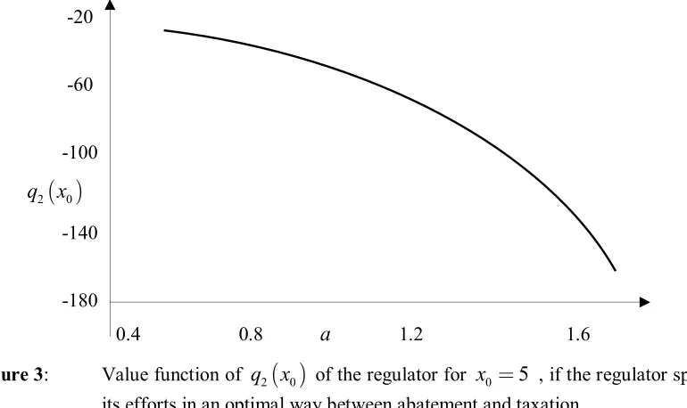
   . Careful inspection in Figure 3, which follows, reveals that the

derivative q x₂

 

₀ a is negative and therefore the partial derivative * 1 a 

  has to be

Proposition 2.

The more efficient the polluting firms are, the smaller is the influence of the current stock of

pollutants on the costs of the regulator.

-20

-60 -100 q x₂

 

₀ -140

-180

[image:18.595.105.490.164.393.2]

0.4 0.8

a

1.2 1.6

Figure 3: Value function of q x₂

 

₀ of the regulator for

x

₀

5

, if the regulator splits its efforts in an optimal way between abatement and taxation

4.b Efficiency of pollutants abatement

In this subsection we analyze the efficiency of abatement. The quantity that measures

this efficiency is the parameter bwhich appears as the factor in the term

b

 



1 2 that

reduces the pollutants accumulation. For the following analysis purposes we consider the

range of values in the interval between 0,5 and 1,5. In the following Figures 4 and 5 we show,

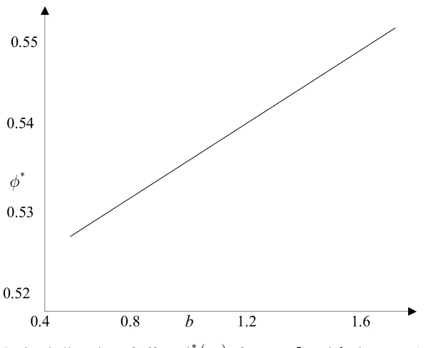
as in the prior subsection, the optimal allocation of efforts _* _{and the long term stock of}

pollutants resulting from an optimal allocation. As we can see the resulting shape between

*

and

b

 is almost linear. The latter reasoning recorded in the following proposition

Proposition 3.

The higher the efficiency of abatement measures, the larger will be the fraction of efforts

invested in abatement.

An increase in parameter b is the cause to a decrease in the long – run stock and therefore to

from abatement is not clear, but by simple inspection of Figure 5 becomes obvious that the

effect from the changing stock is dominant and causes the positive slope of the curve in

Figure 4.

0.55

0.54

_* 0.53

0.52

0.4 0.8 b 1.2 1.6 Figure4: Optimal allocation of efforts *

 

0

x

 for

x

₀



5

and b between 0,5 and 1,5

6.0

4.0

x

* 2.0

[image:19.595.135.437.144.388.2]

0.4 0.8 b 1.2 1.6

[image:19.595.108.491.420.724.2]

We now consider the effect of a decreasing efficiency of the natural recovery, i.e. the

effect of a decreasing efficiency on the decrement of the pollution stock. We have the

following arithmetic results: once parameter b falls down to b=0.5 the value of the pollutants

stock jerks up to

x

*



5.44

_{. The latter implies a strong increase in the costs of the}

government, but however the optimal value of the allocation parameter



reacts intensively

to the changes in parameter b. An increase of b have only a small effect to the stock of

pollutants and decrements the stock’s value approximately 0.5 percent for b=1.5. Therefore

the following result becomes obvious.

Proposition 4.

In the environmental game model as it is defined above, when the stock of pollutants, in the

long – term, becomes a high volume, an increase in abatement effort, on behalf the

government, will have a very large effect on stock.

Conversely for falling stock of pollutants

x

* _{, the marginal effect of increasing parameter b}

diminishes rather rapidly. As the value of the quantity * 2

 represents the cost for government

from one additional unit of pollutants, it is reasonable to discover the effect of changes in this

quantity relative to parameter b, i.e. to discover the partial derivative * 2 b 

  .

Unfortunately, the sign of the latter derivative cannot be determined since two terms with

different signs appear in p_1b and therefore there is no clear statement for the sign.

4.c Efficiency of Taxation measures.

In this case we vary parameter, which measures the efficiency of the taxation

actions, in the interval between 0.5 and 1.5. Again, the figures showing the optimal allocation

between the two efforts _* _{and the optimal stock}

x

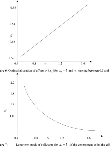
* _{are Figures 6 and 7 respectively.}

As may be seen in Figure 6, at a first glance, it seems rather surprising that an

increase in the efficiency parameter  _{leads to an increase on the optimal allocation}

parameter _*_{. The interpretation is rather straightforward: A higher efficiency of taxation }

firms

u

*_{. Therefore, the marginal utility of abatement process decreases, whereas the} marginal utility of taxation measures increases. In order to balance these effects, the

allocation parameter _* _{has to increase. The impact of the efficiency parameter on taxation}

is not so strong as in the case of the efficiency in abatement. The latter become obvious

since the long – term stock of pollutants varies in the taxation case between 0,7 percent and 2

percent (see Figure 7). Therefore we conclude easily in the following result.

0.55

0.54

_* 0.53

0.52

[image:21.595.106.491.234.744.2]

0.4 0.8  1.2 1.6 Figure 6: Optimal allocation of efforts *

 

0

x

 for

x

₀



5

_and  varying between 0.5 and 1.5

2.2

1.8 1.4

x

* 1.0

[image:21.595.138.425.238.465.2]

0.4 0.8  1.2 1.6

Proposition 5.

The efficiency of taxation measures should have smaller priority to the regulator than the

efficiency of the abatement process.

Now taking the variation of the cost for government from one additional unit of pollutants

with respect to the efficiency parameter of taxation , i.e. * 2

 

  , it is easily seen that

*

2 0

 

   , which means that the costs caused by one additional unit of pollutants at

time 0 increase with increasing  .

5. Conclusions

In this paper, we have analyzed a differential game model between the polluting firms

and the authorities. We believe that the model is kept as simple as possible but some most

important aspects of the pollution abatement as well as polluters’ taxation are incorporated.

With the above game model the government, on one hand, has to decide whether to tackle the

pollution problem from the ‘supply’ side or from the ‘demand’ side. The latter means that the

government has to face the decision whether to decrease the demand for pollutants as much as

possible, or to decrease the supply of pollutants by keeping strong taxation pressure on the

polluting firms.

On the polluters’ side, a major question raised is whether the emissions are profitable

since the polluting firms are faced with the high risk of penalties stemming from taxation.

Turning back into the game, the proposed model is not a trivial case with respect to the

solution process (like the linear quadratic games), but we have been able to find a feedback

Nash equilibrium, i.e. the subgame perfect issue. Since we have found the analytical

expressions of both strategies it is easy to conclude about these.

One major result taken from the strategies is that the polluting firms will strain much

more their effort when the stock of pollutants is small, than in the case they have already built

up a high stock. Another finding is that the same strategy function is a decreasing and convex

more imminent becomes the pollution problem, and the authority’s effort grows linearly with

respect to the stock of pollutants.

Moreover, with this behavior on behalf of the authority, the stock of pollutants tends

to the long-term steady state, a state which is independent of the stock’s initial volume. In the

steady state, the polluting firms strain their effort in order to recover the same volume of

pollutants that are lost due to abatement. In the numerical example that follows, we have seen

that for a farsighted government it is more profitable to invest the larger share of the budget in

abatement and the lower in taxation. In sensitivity analysis we further carry out, one

remarkable thing is the significance of the high efficiency of the abatement process,

undertaken by the government. Conversely, the significance of the taxation measures

becomes of second importance.

Regarding the perspectives on the demand side and on the supply side, a major

conclusion could be that it is recommended for a farsighted authority to deal with the problem

of pollutants from the demand side and put much effort in the abatement process as well as in

the improvement of abatement.

References

Dockner E.J., Jorgensen S., Van Long N. & Sorger G. (2000). Differential games in

economics and management science. Cambridge University Press, Cambridge, UK.

Evangelinos K.I. & Halkos G.E. (2002). Implementation of environmental

management systems standards: important factors in corporate decision making.

Journal of Environmental Assessment Policy and Management,

4(3):

311-328.

Halkos G.E. & Evangelinos K.I. (2002). Determinants of environmental management

systems standards implementation: evidence from Greek industry.

Business Strategy

and the Environment,

11(6):

360-375.

Halkos G.E. (1992). Economic perspectives of the acid rain problem in Europe.

University of York.

Halkos G.E. (1993). Sulphur abatement policy: implications of cost differentials.

Energy Policy,

21(10):

1035-1043.

Halkos G.E. (1994). Optimal abatement of sulphur emissions in Europe.

Environmental and Resource Economics,

4(2):

127-150.

Halkos G.E. & Jones N. (2012). Modeling the effect of social factors on improving

biodiversity protection. Ecological Economics,

78

: 90-99.

Halkos G.E. & Papageorgiou G. (2014). Controlling polluting firms: Nash and

Stackelberg strategies. MPRA Paper

58947

, University Library of Munich, Germany.

Olsder G.J. & Basar T. (1995). Dynamic Non-cooperative Game Theory.

Academic

Press, London, England.