Learning Dependency Based Compositional Semantics

Proceedings of the 49th Annual Meeting of the Association for Computational Linguistics, pages 590–599,

Learning Dependency-Based Compositional Semantics

Percy Liang

UC Berkeley [email protected]

Michael I. Jordan

UC Berkeley [email protected]

Dan Klein

UC Berkeley [email protected]

Abstract

Compositional question answering begins by mapping questions to logical forms, but train-ing a semantic parser to perform this mapptrain-ing typically requires the costly annotation of the target logical forms. In this paper, we learn to map questions to answers via latent log-ical forms, which are induced automatlog-ically from question-answer pairs. In tackling this challenging learning problem, we introduce a new semantic representation which highlights a parallel between dependency syntax and effi-cient evaluation of logical forms. On two stan-dard semantic parsing benchmarks (GEOand JOBS), our system obtains the highest pub-lished accuracies, despite requiring no anno-tated logical forms.

1 Introduction

What is the total population of the ten largest cap-itals in the US?Answering these types of complex questions compositionally involves first mapping the questions into logical forms (semantic parsing). Su-pervised semantic parsers (Zelle and Mooney, 1996; Tang and Mooney, 2001; Ge and Mooney, 2005; Zettlemoyer and Collins, 2005; Kate and Mooney, 2007; Zettlemoyer and Collins, 2007; Wong and Mooney, 2007; Kwiatkowski et al., 2010) rely on manual annotation of logical forms, which is expen-sive. On the other hand, existing unsupervised se-mantic parsers (Poon and Domingos, 2009) do not handle deeper linguistic phenomena such as quan-tification, negation, and superlatives.

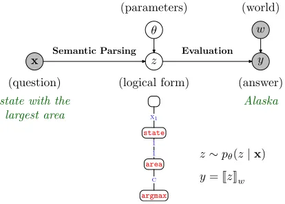
As in Clarke et al. (2010), we obviate the need for annotated logical forms by considering the end-to-end problem of mapping questions to answers. However, we still model the logical form (now as a latent variable) to capture the complexities of lan-guage. Figure 1 shows our probabilistic model:

(parameters) (world)

θ w

x z y

(question) (logical form) (answer)

state with the

largest area xx11

1 1

c c argmax

area state

∗∗ _Alaska

z∼pθ(z|x)

y=_Jz_Kw Semantic Parsing Evaluation

Figure 1: Our probabilistic model: a question x is mapped to a latent logical formz, which is then evaluated with respect to a worldw(database of facts), producing an answer y. We represent logical forms z as labeled trees, induced automatically from(x, y)pairs.

We want to induce latent logical forms z (and pa-rametersθ) given only question-answer pairs(x, y), which is much cheaper to obtain than(x, z)pairs.

The core problem that arises in this setting is pro-gram induction: finding a logical form z (over an exponentially large space of possibilities) that pro-duces the target answery. Unlike standard semantic parsing, our end goal is only to generate the correct

y, so we are free to choose the representation forz. Which one should we use?

Clarke et al. (2010), are simpler but lack the full ex-pressive power of lambda calculus.

The main technical contribution of this work is a new semantic representation, dependency-based compositional semantics(DCS), which is both sim-ple and expressive (Section 2). The logical forms in this framework are trees, which is desirable for two reasons: (i) they parallel syntactic dependency trees, which facilitates parsing and learning; and (ii) eval-uating them to obtain the answer is computationally efficient.

We trained our model using an EM-like algorithm (Section 3) on two benchmarks, GEO and JOBS (Section 4). Our system outperforms all existing systems despite using no annotated logical forms.

2 Semantic Representation

We first present a basic version (Section 2.1) of dependency-based compositional semantics (DCS), which captures the core idea of using trees to rep-resent formal semantics. We then introduce the full version (Section 2.2), which handles linguistic phe-nomena such as quantification, where syntactic and semantic scope diverge.

We start with some definitions, using US geogra-phy as an example domain. LetV be the set of all values, which includes primitives (e.g.,3,CA ∈ V) as well as sets and tuples formed from other values (e.g., 3,{3,4,7},(CA,{5}) ∈ V). Let P be a set ofpredicates(e.g.,state,count ∈ P), which are just symbols.

A world wis mapping from each predicate p ∈ P to a set of tuples; for example, w(state) = {(CA),(OR), . . .}. Conceptually, a world is a rela-tional database where each predicate is a relation (possibly infinite). Define a special predicate ø with

w(ø) =V. We represent functions by a set of input-output pairs, e.g.,w(count) = {(S, n) :n=|S|}. As another example, w(average) = {(S,x¯) : ¯

x = |S1|−1P_x∈S1S(x)}, where a set of pairs S is treated as a set-valued function S(x) = {y : (x, y)∈S}with domainS1={x: (x, y)∈S}.

The logical forms in DCS are called DCS trees, where nodes are labeled with predicates, and edges are labeled with relations. Formally:

Definition 1 (DCS trees) Let Z be the set of DCS trees, where eachz ∈ Z consists of (i) a predicate

RelationsR j

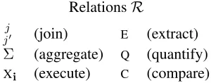
j0 (join) E (extract) Σ (aggregate) Q (quantify) Xi (execute) C (compare)

Table 1: Possible relations appearing on the edges of a DCS tree. Here,j, j0∈ {1,2, . . .}andi∈ {1,2, . . .}∗.

z.p∈ Pand (ii) a sequence of edgesz.e1, . . . , z.em,

each edge econsisting of a relation e.r ∈ R (see Table 1) and a child treee.c∈ Z.

We write a DCS treezashp;r1 :c1;. . .;rm:cmi.

Figure 2(a) shows an example of a DCS tree. Al-though a DCS tree is a logical form, note that it looks like a syntactic dependency tree with predicates in place of words. It is this transparency between syn-tax and semantics provided by DCS which leads to a simple and streamlined compositional semantics suitable for program induction.

2.1 Basic Version

The basic version of DCS restrictsRto join and ag-gregate relations (see Table 1). Let us start by con-sidering a DCS treezwith only join relations. Such az defines a constraint satisfaction problem (CSP) with nodes as variables. The CSP has two types of constraints: (i) x ∈ w(p) for each node x labeled with predicatep ∈ P; and (ii)xj = yj0 (the j-th

component ofx must equal thej0-th component of

y) for each edge(x, y)labeled with_jj0∈ R.

A solution to the CSP is an assignment of nodes to values that satisfies all the constraints. We say a value v is consistent for a node x if there exists a solution that assignsvtox. Thedenotation_Jz_Kw(z

evaluated onw) is the set of consistent values of the root node (see Figure 2 for an example).

Computation We can compute the denotation

JzKw of a DCS tree z by exploiting dynamic

pro-gramming on trees (Dechter, 2003). The recurrence is as follows:

J

D

p;j1

j01:c1;· · · ;

jm jm0 :cm

E

K

w (1)

=w(p)∩ m

\

i=1

{v:vji =tj0

i, t∈JciKw}.

Example: major city in California

z=hcity;11:hmajori;11:hloc;21:hCAiii

1 1 1 1

major

2 1

CA loc city

λc∃m∃`∃s .

city(c)∧major(m)∧

loc(`)∧CA(s)∧

c1=m1∧c1=`1∧`2=s1

(a) DCS tree (b) Lambda calculus formula

(c) Denotation: _Jz_Kw={SF,LA, . . .}

Figure 2: (a) An example of a DCS tree (written in both the mathematical and graphical notation). Each node is labeled with a predicate, and each edge is labeled with a relation. (b) A DCS treez with only join relations en-codes a constraint satisfaction problem. (c) The denota-tion ofzis the set of consistent values for the root node.

for each childi, theji-th component ofvmust equal

the j_i0-th component of some tin the child’s deno-tation (t ∈ _JciKw). This algorithm is linear in the

number of nodes times the size of the denotations.1 Now the dual importance of trees in DCS is clear: We have seen that trees parallel syntactic depen-dency structure, which will facilitate parsing. In addition, trees enable efficient computation, thereby establishing a new connection between dependency syntax and efficient semantic evaluation.

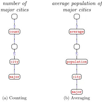
Aggregate relation DCS trees that only use join relations can represent arbitrarily complex compo-sitional structures, but they cannot capture higher-order phenomena in language. For example, con-sider the phrasenumber of major cities, and suppose that number corresponds to the count predicate. It is impossible to represent the semantics of this phrase with just a CSP, so we introduce a new ag-gregate relation, notatedΣ. Consider a treehΣ :ci, whose root is connected to a childcviaΣ. If the de-notation ofcis a set of valuess, the parent’s denota-tion is then a singleton set containings. Formally:

JhΣ :ciKw ={JcKw}. (2)

Figure 3(a) shows the DCS tree for our running example. The denotation of the middle node is{s},

1

Infinite denotations (such asJ<Kw) are represented as

im-plicit sets on which we can perform membership queries. The intersection of two sets can be performed as long as at least one of the sets is finite.

number of major cities

1 2

1 1

Σ Σ

1 1 major

city ∗∗ count

∗∗

average population of major cities

1 2

1 1

Σ Σ

1 1

1 1 major

city population

∗∗ average

∗∗

(a) Counting (b) Averaging

Figure 3: Examples of DCS trees that use the aggregate relation (Σ) to (a) compute the cardinality of a set and (b) take the average over a set.

wheresis all major cities. Having instantiatedsas a value, everything above this node is an ordinary CSP:s constrains thecount node, which in turns constrains the root node to|s|.

A DCS tree that contains only join and aggre-gate relations can be viewed as a collection of tree-structured CSPs connected via aggregate relations. The tree structure still enables us to compute deno-tations efficiently based on (1) and (2).

2.2 Full Version

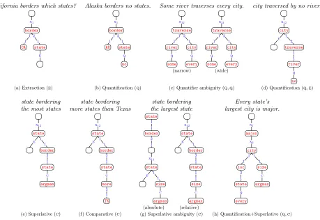
The basic version of DCS described thus far han-dles a core subset of language. But consider Fig-ure 4: (a) is headed by borders, but states needs to be extracted; in (b), the quantifierno is syntacti-cally dominated by the head verbbordersbut needs to take wider scope. We now present the full ver-sion of DCS which handles this type of divergence between syntactic and semantic scope.

The key idea that allows us to give semantically-scoped denotations to syntactically-semantically-scoped trees is as follows: We mark a node low in the tree with a mark relation(one ofE,Q, orC). Then higher up in the tree, we invoke it with anexecute relationX_ito create the desired semantic scope.2

This mark-execute construct acts non-locally, so to maintain compositionality, we must augment the

2

California borders which states? x1 x1 2 1 1 1 CA e e ∗∗ state border ∗∗

Alaska borders no states.

x1 x1 2 1 1 1 AK q q no state border ∗∗

Some river traverses every city.

x12 x12 2 1 1 1 q q some river q q every city traverse ∗∗ x21 x21 2 1 1 1 q q some river q q every city traverse ∗∗ (narrow) (wide)

city traversed by no rivers

x12 x12 1 2 e e ∗∗ 1 1 q q no river traverse city ∗∗

(a) Extraction (e) (b) Quantification (q) (c) Quantifier ambiguity (q,q) (d) Quantification (q,e)

state bordering the most states

x12 x12 1 1 e e ∗∗ 2 1 c c argmax state border state ∗∗ state bordering more states than Texas

x12 x12 1 1 e e ∗∗ 2 1 c c 3 1 TX more state border state ∗∗ state bordering the largest state

1 1 2 1 x12 x12 1 1 e e ∗∗ c c argmax size state ∗∗ border state x12 x12 1 1 e e ∗∗ 2 1 1 1 c c argmax size state border state ∗∗ (absolute) (relative) Every state’s largest city is major.

x1 x1 x2 x2 1 1 1 1 2 1 q q every state loc c c argmax size city major ∗∗

(e) Superlative (c) (f) Comparative (c) (g) Superlative ambiguity (c) (h) Quantification+Superlative (q,c)

Figure 4: Example DCS trees for utterances in which syntactic and semantic scope diverge. These trees reflect the syntactic structure, which facilitates parsing, but importantly, these trees also precisely encode the correct semantic scope. The main mechanism is using a mark relation (E,Q, orC) low in the tree paired with an execute relation (Xi)

higher up at the desired semantic point.

denotation d = _Jz_Kw to include any information about the marked nodes in z that can be accessed by an execute relation later on. In the basic ver-sion,dwas simply the consistent assignments to the root. Now d contains the consistent joint assign-ments to the active nodes (which include the root and all marked nodes), as well as information stored about each marked node. Think of das consisting ofncolumns, one for each active node according to a pre-order traversal ofz. Column 1 always corre-sponds to the root node. Formally, a denotation is defined as follows (see Figure 5 for an example):

Definition 2 (Denotations) Let Dbe the set of de-notations, where eachd∈ Dconsists of

• a set of arrays d.A, where each array a = [a1, . . . , an] ∈ d.A is a sequence of n tuples

(ai∈ V∗); and

• a list of n stores d.α = (d.α1, . . . , d.αn),

where each store α contains a mark relation

α.r ∈ {E,Q,C,ø}, a base denotation α.b ∈ D ∪ {ø}, and a child denotationα.c∈ D ∪ {ø}.

We writedashhA; (r1, b1, c1);. . .; (rn, bn, cn)ii. We

used{ri = x}to mean dwith d.ri = d.αi.r = x

(similar definitions apply ford{αi=x},d{bi =x},

andd{ci =x}).

The denotation of a DCS tree can now be defined recursively:

JhpiKw =hh{[v] :v∈w(p)};øii, (3)

J

D

p;e;_jj0:c

E

K

w =Jp;eKw./j,j

0

JcKw, (4)

Jhp;e; Σ :ciKw =Jp;eKw./∗,∗Σ (JcKw), (5)

Jhp;e;Xi:ciKw =Jp;eKw./∗,∗Xi(JcKw), (6)

Jhp;e;E:ciKw =M(Jp;eKw,E, c), (7)

Jhp;e;C:ciKw =M(Jp;eKw,C, c), (8)

1 1

2 1

1 1

c c

argmax size state border state

J·Kw

column 1 column 2

A: (OK) (NM) (NV)

· · ·

(TX,2.7e5) (TX,2.7e5) (CA,1.6e5)

· · ·

r: ø c

b: ø JhsizeiKw

c: ø _Jhargmaxi_Kw

DCS tree Denotation

Figure 5: Example of the denotation for a DCS tree with a compare relationC. This denotation has two columns, one for each active node—the root nodestateand the marked nodesize.

The base case is defined in (3): if z is a sin-gle node with predicatep, then the denotation of z

has one column with the tuplesw(p)and an empty store. The other six cases handle different edge re-lations. These definitions depend on several opera-tions (./j,j0,Σ,X_i,M) which we will define shortly,

but let us first get some intuition.

Let z be a DCS tree. If the last child c of z’s root is a join (_jj0), aggregate (Σ), or execute (X_i)

re-lation ((4)–(6)), then we simply recurse onzwithc

removed and join it with some transformation (iden-tity,Σ, orXi) ofc’s denotation. If the last (or first)

child is connected via a mark relation E,C (or Q), then we strip off that child and put the appropriate information in the store by invokingM.

We now define the operations ./j,j0,Σ,X_i,M.

Some helpful notation: For a sequence v = (v1, . . . , vn) and indices i = (i1, . . . , ik), let vi = (vi1, . . . , vik)be the projection ofvontoi; we write

v−i to mean v[1,...,n]\i. Extending this notation to

denotations, lethhA;αii[i] = hh{ai : a ∈ A};αiii.

Let d[−ø] = d[−i], where i are the columns with empty stores. For example, for din Figure 5,d[1]

keeps column 1,d[−ø]keeps column 2, andd[2,−2]

swaps the two columns.

Join Thejoinof two denotationsdandd0 with re-spect to components j and j0 (∗ means all compo-nents) is formed by concatenating all arraysa ofd

with all compatible arraysa0 ofd0, where compat-ibility meansa1j = a01j0. The stores are also

con-catenated (α+α0). Non-initial columns with empty stores are projected away by applying·[1,−ø]. The

full definition of join is as follows:

hhA;αii./j,j0 hhA0;α0ii=hhA00;α+α0ii[1,−ø],

A00={a+a0 :a∈A,a0∈A0, a1j=a01j0}. (10)

Aggregate The aggregate operation takes a deno-tation and forms a set out of the tuples in the first column for each setting of the rest of the columns:

Σ (hhA;αii) =hhA0∪A00;αii (11)

A0={[S(a), a2, . . . , an] :a∈A}

S(a) ={a0₁ : [a0₁, a2, . . . , an]∈A}

A00={[∅, a2, . . . , an] :¬∃a1,a∈A,

∀2≤i≤n,[ai]∈d.bi[1].A}.

2.2.1 Mark and Execute

Now we turn to the mark (M) and execute (Xi)

operations, which handles the divergence between syntactic and semantic scope. In some sense, this is the technical core of DCS. Marking is simple: When a node (e.g.,sizein Figure 5) is marked (e.g., with relationC), we simply put the relationr, current de-notationdand childc’s denotation into the store of column 1:

M(d, r, c) =d{r1 =r, b1 =d, c1 =JcKw}. (12)

The execute operation Xi(d) processes columns i in reverse order. It suffices to defineXi(d) for a

single columni. There are three cases:

Extraction (d.ri = E) In the basic version, the

denotation of a tree was always the set of con-sistent values of the root node. Extraction al-lows us to return the set of consistent values of a marked non-root node. Formally, extraction sim-ply moves the i-th column to the front: Xi(d) =

d[i,−(i,ø)]{α1 =ø}. For example, in Figure 4(a),

before execution, the denotation of the DCS tree is hh{[(CA,OR),(OR)], . . .};ø; (E,JhstateiKw,ø)ii;

after applyingX1, we havehh{[(OR)], . . .};øii.

Generalized Quantification (d.ri = Q)

Gener-alized quantifiers are predicates on two sets, a re-strictor A and a nuclear scope B. For example,

w(no) = {(A, B) : A∩B = ∅}andw(most) = {(A, B) :|A∩B|> 1₂|A|}.

quantifier in column i is executed. In particu-lar, the restrictor is A = Σ (d.bi) and the

nu-clear scope is B = Σ (d[i,−(i,ø)]). We then apply d.ci to these two sets (technically,

denota-tions) and project away the first column: Xi(d) =

((d.ci./1,1 A)./2,1 B) [−1].

For the example in Figure 4(b), the de-notation of the DCS tree before execution is

hh∅;ø; (Q,_Jhstatei_Kw,_Jhnoi_Kw)ii. The restrictor set (A) is the set of all states, and the nuclear scope (B) is the empty set. Since(A, B)exists inno, the final denotation, which projects away the actual pair, ishh{[ ]}ii(our representation of true).

Figure 4(c) shows an example with two interact-ing quantifiers. The quantifier scope ambiguity is resolved by the choice of execute relation;X12gives

the narrow reading and X21 gives the wide reading.

Figure 4(d) shows how extraction and quantification work together.

Comparatives and Superlatives (d.ri = C) To

compare entities, we use a set S of (x, y) pairs, where x is an entity and y is a number. For su-perlatives, the argmax predicate denotes pairs of sets and the set’s largest element(s): w(argmax) = {(S, x∗) : x∗ ∈ argmax_x∈S1maxS(x)}. For com-paratives,w(more)contains triples(S, x, y), where

x is “more than” y as measured by S; formally:

w(more) ={(S, x, y) : maxS(x)>maxS(y)}. In a superlative/comparative construction, the rootxof the DCS tree is the entity to be compared, the childcof aCrelation is the comparative or su-perlative, and its parentp contains the information used for comparison (see Figure 4(e) for an exam-ple). Ifdis the denotation of the root, itsi-th column contains this information. There are two cases: (i) if the i-th column of dcontains pairs (e.g., size in Figure 5), then letd0 =_Jhøi_Kw ./1,2 d[i,−i], which

reads out the second components of these pairs; (ii) otherwise (e.g., state in Figure 4(e)), let d0 =

JhøiKw ./1,2 JhcountiKw ./1,1 Σ (d[i,−i]), which

counts the number of things (e.g., states) that occur with each value of the rootx. Givend0, we construct a denotationSby concatenating (+i) the second and

first columns of d0 (S = Σ (+2,1(d0{α2=ø})))

and apply the superlative/comparative: Xi(d) =

(_Jhøi_Kw ./1,2(d.ci./1,1 S)){α1 =d.α1}.

Figure 4(f) shows that comparatives are handled

using the exact same machinery as superlatives. Fig-ure 4(g) shows that we can naturally account for superlative ambiguity based on where the scope-determining execute relation is placed.

3 Semantic Parsing

We now turn to the task of mapping natural language utterances to DCS trees. Our first question is: given an utterancex, what treesz∈ Zare permissible? To define the search space, we first assume a fixed set oflexical triggers L. Each trigger is a pair (x, p), wherexis a sequence of words (usually one) andp

is a predicate (e.g., x = California andp = CA). We useL(x)to denote the set of predicatesp trig-gered by x ((x, p) ∈ L). Let L() be the set of trace predicates, which can be introduced without an overt lexical trigger.

Given an utterance x = (x1, . . . , xn), we define ZL(x) ⊂ Z, the set of permissible DCS trees for x. The basic approach is reminiscent of projective labeled dependency parsing: For each spani..j, we build a set of treesCi,j and setZL(x) =C0,n. Each

setCi,j is constructed recursively by combining the

trees of its subspansCi,k andCk0_,j for each pair of

split points k, k0 (words between k and k0 are ig-nored). These combinations are then augmented via a functionAand filtered via a functionF, to be spec-ified later. Formally, Ci,j is defined recursively as

follows:

Ci,j =F

A

L(xi+1..j)∪

[

i≤k≤k0<j a∈Ci,k b∈Ck0,j

T1(a, b))

.

(13)

In (13),L(xi+1..j) is the set of predicates triggered

by the phrase under span i..j (the base case), and

Td(a, b) = T~d(a, b) ∪ ~Td(b, a), which returns all

ways of combining trees a and b where b is a de-scendant ofa(T~d) or vice-versa ( ~Td). The former is

defined recursively as follows:T~0(a, b) =∅, and

~

Td(a, b) =

[

r∈R p∈L()

{ha;r:bi} ∪T~d−1(a,hp;r:bi).

The latter ( ~Tk) is defined similarly. Essentially,

~

Td(a, b) allows us to insert up to d trace

California cities), and it also allows us to underspec-ifyL. In particular, ourLwill not include verbs or prepositions; rather, we rely on the predicates corre-sponding to those words to be triggered by traces.

The augmentation functionAtakes a set of trees and optionally attaches E and Xi relations to the

root (e.g., A(hcityi) = {hcityi,hcity;E:øi}). The filtering functionF rules out improperly-typed trees such ashcity;0

0:hstateii. To further reduce

the search space, F imposes a few additional con-straints, e.g., limiting the number of marked nodes to 2 and only allowing trace predicates between ar-ity 1 predicates.

Model We now present our discriminative se-mantic parsing model, which places a log-linear distribution over z ∈ Z_L(x) given an utter-ance x. Formally, pθ(z | x) ∝ eφ(x,z)

>_θ

, whereθandφ(x, z)are parameter and feature vec-tors, respectively. As a running example, con-sider x = city that is in California and z = hcity;1

1:hloc;21:hCAiii, where citytriggers city

andCaliforniatriggersCA.

To define the features, we technically need to augment each tree z ∈ ZL(x) with alignment

information—namely, for each predicate in z, the span inx(if any) that triggered it. This extra infor-mation is already generated from the recursive defi-nition in (13).

The feature vectorφ(x, z) is defined by sums of five simple indicator feature templates: (F1) a word

triggers a predicate (e.g.,[city,city]); (F2) a word

is under a relation (e.g.,[that,1

1]); (F3) a word is

un-der a trace predicate (e.g.,[in,loc]); (F4) two

pred-icates are linked via a relation in the left or right direction (e.g., [city,1

1,loc,RIGHT]); and (F5) a

predicate has a child relation (e.g.,[city,1₁]).

Learning Given a training dataset D con-taining (x, y) pairs, we define the regu-larized marginal log-likelihood objective

O(θ) = P

(x,y)∈Dlogpθ(JzKw = y | x, z ∈ ZL(x))−λkθk22, which sums over all DCS treesz

that evaluate to the target answery.

Our model is arc-factored, so we can sum over all DCS trees in Z_L(x) using dynamic programming. However, in order to learn, we need to sum over

{z ∈ ZL(x) : JzKw = y}, and unfortunately, the

additional constraint _Jz_Kw = y does not factorize. We therefore resort to beam search. Specifically, we truncate eachCi,j to a maximum of K candidates

sorted by decreasing score based on parameters θ. LetZ˜_L,θ(x)be this approximation ofZ_L(x).

Our learning algorithm alternates between (i) us-ing the current parametersθto generate theK-best set Z˜_L,θ(x) for each training example x, and (ii) optimizing the parameters to put probability mass on the correct trees in these sets; sets contain-ing no correct answers are skipped. Formally, let

˜

O(θ, θ0)be the objective functionO(θ)withZ_L(x)

replaced with Z˜L,θ0(x). We optimize O˜(θ, θ0) by

setting θ(0) = ~0 and iteratively solving θ(t+1) =

argmax_θO˜(θ, θ(t))using L-BFGS untilt=T. In all experiments, we setλ= 0.01,T = 5, andK = 100. After training, given a new utterancex, our system outputs the most likely y, summing out the latent logical formz: argmax_yp_θ(T)(y|x, z ∈Z˜_L,θ(T)).

4 Experiments

We tested our system on two standard datasets, GEO and JOBS. In each dataset, each sentence xis an-notated with a Prolog logical form, which we use only to evaluate and get an answery. This evalua-tion is done with respect to a world w. Recall that a world w maps each predicate p ∈ P to a set of tuplesw(p). There are three types of predicates in

P: generic (e.g., argmax), data (e.g., city), and value (e.g., CA). GEO has 48 non-value predicates and JOBS has 26. For GEO, w is the standard US geography database that comes with the dataset. For JOBS, if we use the standard Jobs database, close to half they’s are empty, which makes it uninteresting. We therefore generated a random Jobs database in-stead as follows: we created 100 job IDs. For each data predicatep(e.g.,language), we add each pos-sible tuple (e.g., (job37,Java)) tow(p) indepen-dently with probability 0.8.

We used the same training-test splits as Zettle-moyer and Collins (2005) (600+280 for GEO and 500+140 for JOBS). During development, we fur-ther held out a random 30% of the training sets for validation.

System Accuracy Clarke et al. (2010) w/answers 73.2 Clarke et al. (2010) w/logical forms 80.4 Our system (DCS withL) 78.9 Our system (DCS withL+) 87.2

Table 2: Results on GEO with 250 training and 250 test examples. Our results are averaged over 10 random 250+250 splits taken from our 600 training examples. Of the three systems that do not use logical forms, our two systems yield significant improvements. Our better sys-tem even outperforms the syssys-tem that uses logical forms.

predicate x in w (e.g., (Boston,Boston)), and (iii) predicates for each POS tag in {JJ,NN,NNS} (e.g., (JJ,size), (JJ,area), etc.).3 Predicates corresponding to verbs and prepositions (e.g.,

traverse) are not included as overt lexical

trig-gers, but rather in the trace predicatesL().

We also define an augmented lexicon L+ which includes a prototype wordx for each predicate ap-pearing in (iii) above (e.g., (large,size)), which cancels the predicates triggered byx’s POS tag. For GEO, there are 22 prototype words; for JOBS, there are 5. Specifying these triggers requires minimal domain-specific supervision.

Results We first compare our system with Clarke et al. (2010) (henceforth, SEMRESP), which also learns a semantic parser from question-answer pairs. Table 2 shows that our system using lexical triggers

L(henceforth,DCS) outperforms SEMRESP(78.9% over 73.2%). In fact, although neither DCS nor SEMRESPuses logical forms,DCSuses even less su-pervision than SEMRESP. SEMRESPrequires a lex-icon of 1.42 words per non-value predicate, Word-Net features, and syntactic parse trees;DCSrequires only words for the domain-independent predicates (overall, around 0.5 words per non-value predicate), POS tags, and very simple indicator features. In fact, DCS performs comparably to even the version of SEMRESPtrained using logical forms. If we add prototype triggers (use L+), the resulting system (DCS+) outperforms both versions of SEMRESP by a significant margin (87.2% over 73.2% and 80.4%).

3

We used the Berkeley Parser (Petrov et al., 2006) to per-form POS tagging. The triggersL(x)for a wordxthus include

L(t)wheretis the POS tag ofx.

System GEO JOBS

Tang and Mooney (2001) 79.4 79.8 Wong and Mooney (2007) 86.6 – Zettlemoyer and Collins (2005) 79.3 79.3 Zettlemoyer and Collins (2007) 81.6 – Kwiatkowski et al. (2010) 88.2 – Kwiatkowski et al. (2010) 88.9 – Our system (DCS withL) 88.6 91.4 Our system (DCS withL+_{) 91.1 95.0}

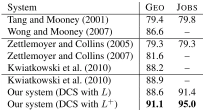
Table 3: Accuracy (recall) of systems on the two bench-marks. The systems are divided into three groups. Group 1 uses 10-fold cross-validation; groups 2 and 3 use the in-dependent test set. Groups 1 and 2 measure accuracy of logical form; group 3 measures accuracy of the answer; but there is very small difference between the two as seen from the Kwiatkowski et al. (2010) numbers. Our best system improves substantially over past work, despite us-ing no logical forms as trainus-ing data.

Next, we compared our systems (DCSandDCS+) with the state-of-the-art semantic parsers on the full dataset for both GEO and JOBS (see Table 3). All other systems require logical forms as training data, whereas ours does not. Table 3 shows that evenDCS, which does not use prototypes, is comparable to the best previous system (Kwiatkowski et al., 2010), and by adding a few prototypes,DCS+offers a decisive edge (91.1% over 88.9% on GEO). Rather than us-ing lexical triggers, several of the other systems use IBM word alignment models to produce an initial word-predicate mapping. This option is not avail-able to us since we do not have annotated logical forms, so we must instead rely on lexical triggers to define the search space. Note that having lexical triggers is a much weaker requirement than having a CCG lexicon, and far easier to obtain than logical forms.

model to generate the correct answer using any tree. Our system learns lexical associations between words and predicates. For example,area (by virtue of being a noun) triggers many predicates: city,

state, area, etc. Inspecting the final parameters

(DCSon GEO), we find that the feature[area,area]

has a much higher weight than[area,city]. Trace predicates can be inserted anywhere, but the fea-tures favor some insertions depending on the words present (for example,[in,loc]has high weight).

The errors that the system makes stem from mul-tiple sources, including errors in the POS tags (e.g., statesis sometimes tagged as a verb, which triggers no predicates), confusion of Washington state with Washington D.C., learning the wrong lexical asso-ciations due to data sparsity, and having an insuffi-ciently largeK.

5 Discussion

A major focus of this work is on our semantic rep-resentation, DCS, which offers a new perspective on compositional semantics. To contrast, consider CCG (Steedman, 2000), in which semantic pars-ing is driven from the lexicon. The lexicon en-codes information about how each word can used in context; for example, the lexical entry for borders is S\NP/NP : λy.λx.border(x, y), which means borders looks right for the first argument and left for the second. These rules are often too stringent, and for complex utterances, especially in free word-order languages, either disharmonic combinators are employed (Zettlemoyer and Collins, 2007) or words are given multiple lexical entries (Kwiatkowski et al., 2010).

In DCS, we start with lexical triggers, which are more basic than CCG lexical entries. A trigger for bordersspecifies only thatbordercan be used, but not how. The combination rules are encoded in the features as soft preferences. This yields a more factorized and flexible representation that is easier to search through and parametrize using features. It also allows us to easily add new lexical triggers without becoming mired in the semantic formalism. Quantifiers and superlatives significantly compli-cate scoping in lambda calculus, and often type rais-ing needs to be employed. In DCS, the mark-execute construct provides a flexible framework for dealing

with scope variation. Think of DCS as a higher-level programming language tailored to natural language, which results in programs (DCS trees) which are much simpler than the logically-equivalent lambda calculus formulae.

The idea of using CSPs to represent semantics is inspired by Discourse Representation Theory (DRT) (Kamp and Reyle, 1993; Kamp et al., 2005), where variables are discourse referents. The restriction to trees is similar to economical DRT (Bos, 2009).

The other major focus of this work is program induction—inferring logical forms from their deno-tations. There has been a fair amount of past work on this topic: Liang et al. (2010) induces combinatory logic programs in a non-linguistic setting. Eisen-stein et al. (2009) induces conjunctive formulae and uses them as features in another learning problem. Piantadosi et al. (2008) induces first-order formu-lae using CCG in a small domain assuming observed lexical semantics. The closest work to ours is Clarke et al. (2010), which we discussed earlier.

The integration of natural language with denota-tions computed against a world (grounding) is be-coming increasingly popular. Feedback from the world has been used to guide both syntactic parsing (Schuler, 2003) and semantic parsing (Popescu et al., 2003; Clarke et al., 2010). Past work has also fo-cused on aligning text to a world (Liang et al., 2009), using text in reinforcement learning (Branavan et al., 2009; Branavan et al., 2010), and many others. Our work pushes the grounded language agenda towards deeper representations of language—think grounded compositional semantics.

6 Conclusion

We built a system that interprets natural language utterances much more accurately than existing sys-tems, despite using no annotated logical forms. Our system is based on a new semantic representation, DCS, which offers a simple and expressive alter-native to lambda calculus. Free from the burden of annotating logical forms, we hope to use our techniques in developing even more accurate and broader-coverage language understanding systems.

References

J. Bos. 2009. A controlled fragment of DRT. In Work-shop on Controlled Natural Language, pages 1–5. S. Branavan, H. Chen, L. S. Zettlemoyer, and R. Barzilay.

2009. Reinforcement learning for mapping instruc-tions to acinstruc-tions. InAssociation for Computational Lin-guistics and International Joint Conference on Natural Language Processing (ACL-IJCNLP), Singapore. As-sociation for Computational Linguistics.

S. Branavan, L. Zettlemoyer, and R. Barzilay. 2010. Reading between the lines: Learning to map high-level instructions to commands. InAssociation for Compu-tational Linguistics (ACL). Association for Computa-tional Linguistics.

B. Carpenter. 1998.Type-Logical Semantics. MIT Press. J. Clarke, D. Goldwasser, M. Chang, and D. Roth. 2010. Driving semantic parsing from the world’s re-sponse. InComputational Natural Language Learn-ing (CoNLL).

R. Dechter. 2003.Constraint Processing. Morgan Kauf-mann.

J. Eisenstein, J. Clarke, D. Goldwasser, and D. Roth. 2009. Reading to learn: Constructing features from semantic abstracts. In Empirical Methods in Natural Language Processing (EMNLP), Singapore.

R. Ge and R. J. Mooney. 2005. A statistical semantic parser that integrates syntax and semantics. In Compu-tational Natural Language Learning (CoNLL), pages 9–16, Ann Arbor, Michigan.

H. Kamp and U. Reyle. 1993. From Discourse to Logic: An Introduction to the Model-theoretic Semantics of Natural Language, Formal Logic and Discourse Rep-resentation Theory. Kluwer, Dordrecht.

H. Kamp, J. v. Genabith, and U. Reyle. 2005. Discourse representation theory. InHandbook of Philosophical Logic.

R. J. Kate and R. J. Mooney. 2007. Learning lan-guage semantics from ambiguous supervision. In As-sociation for the Advancement of Artificial Intelligence (AAAI), pages 895–900, Cambridge, MA. MIT Press. R. J. Kate, Y. W. Wong, and R. J. Mooney. 2005.

Learning to transform natural to formal languages. In

Association for the Advancement of Artificial Intel-ligence (AAAI), pages 1062–1068, Cambridge, MA. MIT Press.

T. Kwiatkowski, L. Zettlemoyer, S. Goldwater, and M. Steedman. 2010. Inducing probabilistic CCG grammars from logical form with higher-order unifi-cation. In Empirical Methods in Natural Language Processing (EMNLP).

P. Liang, M. I. Jordan, and D. Klein. 2009. Learning se-mantic correspondences with less supervision. In As-sociation for Computational Linguistics and

Interna-tional Joint Conference on Natural Language Process-ing (ACL-IJCNLP), Singapore. Association for Com-putational Linguistics.

P. Liang, M. I. Jordan, and D. Klein. 2010. Learning programs: A hierarchical Bayesian approach. In In-ternational Conference on Machine Learning (ICML). Omnipress.

S. Petrov, L. Barrett, R. Thibaux, and D. Klein. 2006. Learning accurate, compact, and interpretable tree an-notation. In International Conference on Computa-tional Linguistics and Association for ComputaComputa-tional Linguistics (COLING/ACL), pages 433–440. Associa-tion for ComputaAssocia-tional Linguistics.

S. T. Piantadosi, N. D. Goodman, B. A. Ellis, and J. B. Tenenbaum. 2008. A Bayesian model of the acquisi-tion of composiacquisi-tional semantics. InProceedings of the Thirtieth Annual Conference of the Cognitive Science Society.

H. Poon and P. Domingos. 2009. Unsupervised semantic parsing. InEmpirical Methods in Natural Language Processing (EMNLP), Singapore.

A. Popescu, O. Etzioni, and H. Kautz. 2003. Towards a theory of natural language interfaces to databases. InInternational Conference on Intelligent User Inter-faces (IUI).

W. Schuler. 2003. Using model-theoretic semantic inter-pretation to guide statistical parsing and word recog-nition in a spoken language interface. InAssociation for Computational Linguistics (ACL). Association for Computational Linguistics.

M. Steedman. 2000. The Syntactic Process. MIT Press. L. R. Tang and R. J. Mooney. 2001. Using multiple

clause constructors in inductive logic programming for semantic parsing. In European Conference on Ma-chine Learning, pages 466–477.

Y. W. Wong and R. J. Mooney. 2007. Learning syn-chronous grammars for semantic parsing with lambda calculus. InAssociation for Computational Linguis-tics (ACL), pages 960–967, Prague, Czech Republic. Association for Computational Linguistics.

M. Zelle and R. J. Mooney. 1996. Learning to parse database queries using inductive logic proramming. In

Association for the Advancement of Artificial Intelli-gence (AAAI), Cambridge, MA. MIT Press.

L. S. Zettlemoyer and M. Collins. 2005. Learning to map sentences to logical form: Structured classifica-tion with probabilistic categorial grammars. In Uncer-tainty in Artificial Intelligence (UAI), pages 658–666. L. S. Zettlemoyer and M. Collins. 2007. Online