Altered Jacobian Newton Iterative Method for Nonlinear Elliptic Problems

Altered Jacobian Newton Iterative Method for

Nonlinear Elliptic Problems

Sanjay K. Khattri

Abstract—We present an Altered Jacobian New-ton Iterative Method for solving nonlinear elliptic problems. Effectiveness of the proposed method is demonstrated through numerical experiments. Com-parison of our method with Newton Iterative Method is also presented. Convergence of the Newton Itera-tive Method is highly sensiItera-tive to the initialization or initial guess. Reported numerical work shows the robustness of the Altered Jacobian Newton Iterative Method with respect to initialization.

Keywords: Newton, Jacobian, non-linear, elliptic, Krylov solver

1

Introduction

The past fifty to sixty years have seen a considerable

ad-vancement in methods for solving linear systems. Krylov

subspace method is the result of the huge effort by the

re-searchers during the last century. It is one among the top

ten algorithms of the 20th century. There exists optimal

linear solvers [5]. But, still there is no optimal nonlinear

solver or the one that we know of. Our research is in the

field of optimal solution of nonlinear equations generated

by the discretization of the nonlinear partial differential

equation [1; 2; 3; 4]. Let us consider the following

non-linear elliptic partial differential equation [4]

div(−K grad_p) +_f(_p) =_s(_{x, y}) _in Ω (1)

p(x, y) =pD on ∂Ω_D (2)

g(_{x, y}) = (−K∇_p)·_nˆ _{on ∂}Ω_N (3)

Here, Ω is a polyhedral domain in Rd (d = 2, 3), the

source function s(x, y) is assumed to be in L2_{(Ω), and}

the medium property K is uniformly positive. In the

equations (2) and (3),_∂Ω_D and_∂Ω_N represent Dirichlet

and Neumann part of the boundary, respectively. _f(_p)

represents nonlinear part of the equation. _p is the

un-known function. The equations (1), (2) and (3) models a

wide variety of processes with practical applications. For

example, pattern formation in biology, viscous fluid flow

phenomena, chemical reactions, biomolecule

electrostat-ics and crystal growth [6; 7; 8; 9; 10; 11].

There are various methods for discretizing the equations

(1), (2) and (3). To mention a few: Finite Volume, Finite

∗_{Address: Stord/Haugesund University College & Haugesund,} Norway Tel/Fax: 52 70 26 83 Email: [email protected]

p25

p13

p5

p1 p2

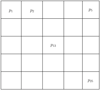
Figure 1: A 5×5 mesh.

Element and Finite Difference methods [1]. These

meth-ods converts nonlinear partial differential equations into

a system of algebraic equations.

Let discretization of the nonlinear partial differential

equations result in a system of nonlinear algebraic

equa-tions_A(_p) = 0. Each cell in the mesh produces a

nonlin-ear algebraic equation [1; 4]. Thus, discretization of the

equations (1), (2) and (3) on a mesh with_ncells result in

n nonlinear equations, and let these equations are given

as

A(_p) =     

A1(p)

A2(p)

. . .

An(p)

   

. (4)

Figure 1 depicts a 5×5 mesh with the unknown_p. Since,

the mesh contains 25 cells. Thus, the vector _A(_p) for

this mesh will consist of 25 nonlinear algebraic equations

[see 4]. In the next section, Altered Jacobian Newton

Iterative Method is presented.

2

Altered

Jacobian

Newton

Iterative

Method

We are interested in finding the vector _p for which the

operator_A(_p) vanish. Let us first formulate the Newton

operator_A(_p) around some initial guess_p0is

A(_p) =_A(_p0) +_J(_p0) ∆_p+_hot, (5)

where _hotstands for higher order terms. That is, terms

involving higher than the first power of ∆_p. Here,

dif-ference vector ∆_p=_p−_p0. The Jacobian_J is a_n×_n

linear system evaluated at the_p0. The Jacobian_J in the

equation (5) is given as follows

J = [ ∂Ai ∂pj ] =             ∂A1 ∂p1 ∂A1

∂p2 · · ·

∂A1 ∂pn ∂A2 ∂p1 ∂A2 ∂p2

· · · ∂A2

∂pn . . . . . . . .. . . . ∂An ∂p1 ∂An

∂p2 · · ·

∂An ∂pn             . (6)

Since, we are interested in the zeroth of the non-linear

vector function _A(_p). Thus, setting the equation (5)

equals to zero and neglecting higher order terms will

re-sult in the following well known Newton Iteration Method

(NIM)

J(pk) ∆pk+1 =−A(pk),

pk+1 =pk+ ∆pk+1, k= 0, . . . , n.

(7)

Newton Iterative Method may not always converge, and

it’s convergence depends on the initialization p0. If the

initial guess if far from the exact solution, the Newton’s

method may not converge.

Let us modify the Jacobian (6) as follows

Jf def=             ∂A1 ∂p1

+_A1(_p1) ∂A1

∂p2 · · ·

∂A1 ∂pn ∂A2 ∂p1 ∂A2 ∂p2

+A2(p2) · · ·

∂A2 ∂pn . . . . . . . .. . . . ∂An ∂p1 ∂An

∂p2 · · ·

∂An

∂pn

+_An(_pn)

            . (8)

Here,_Ai(_pj) is the_ith element of the vector_Aevaluated

at_pj. Based on the above definition of the Altered

Jaco-bian, we propose the following Alterned Jacobian Newton

Iterative Method (AJNIM)

3

Numerical Experimentation

Without loss of generality let us assume that K is unity,

and the boundary is of Dirichlet type. Let _f(_p) be

104_{pexp(p). Thus, the equations (1), (2) and (3) are}

written as

−∇2_{p+ 10}4_{pexp(p) =f in Ω, (10)}

p(x, y) =pD on ∂Ω_D. (11)

For computing the true error and convergence behavior of

the methods, let us further assume that the exact solution

of the equations (10) and (11) is the following bubble

function

p=_x(_x−1)_y(_y−1)_.

Let our domain be a unit square. Thus, Ω = [0,1]×

[0,1]. We are discretizing equations (10) and (11) on a

20×20 mesh by the method of Finite Volumes [1; 2; 4; 12].

Discretization results in a nonlinear algebraic vector (4)

with 400 nonlinear equations.

If the method is convergent, _L2 norm of the difference

vector, ∆_p, and the residual vector, _A(_p), converge to

zero [see 12]. We are reporting convergence of both of

these vectors. For better understanding the error

re-ducing property of these methods, we report variation of

∥A(_pk)∥_L

2/∥A(p0)∥L2 and∥∆(pk)∥L2/∥∆(p0)∥L2 with

iterations (k).

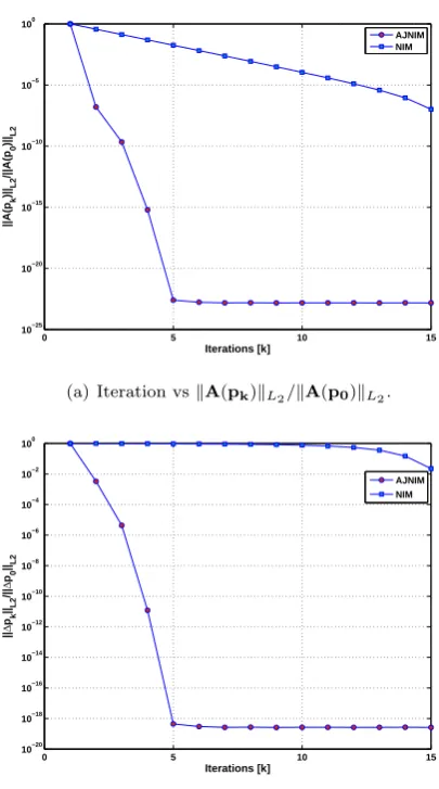
We performed three experiments with different

initializa-tion in the algorithms (7) and (9). In the first test, let the

initial vector be zero for both the algorithms. Figure 2

re-ports the result. Figure 2(a) presents convergence of the

residual vector while the Figure 2(b) presents convergence

of the difference vector. In these figures, NIM stands for

Newton Iterative Method while AJNIM stands for

Al-terted Newton Iterative Method. These figures show that

both the methods converges at the same rate

(quadrat-ically), but still the Altered Jacobian Newton Iterative

Method is better in reducing the error.

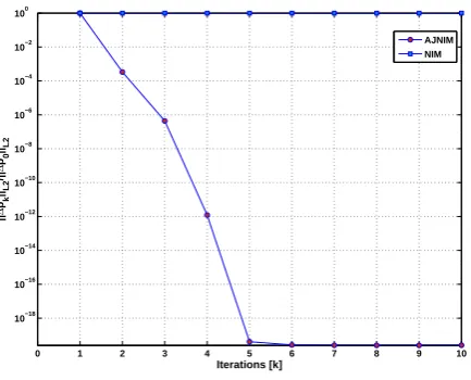
In the second case, let us select initial vector whose

ele-ments 10. Figure 3 presents comparison of the two

meth-ods for an initial vector whose elements are 10. It can be

seen in the Figures 3(a) and 3(b) that the Altered

Jaco-bian Newton Iterative Method converges faster than the

0 1 2 3 4 5 6 7 8 9 10 10−25

10−20 10−15 10−10

10−5 100

Iterations [k]

||A(p

k

)||

L

2

/||A(p

0

)||

L

2

AJNIM

NIM

(a) Iteration vs∥A(pk)∥L2/∥A(p0)∥L2.

0 1 2 3 4 5 6 7 8 9 10

10−18

10−16

10−14

10−12

10−10

10−8

10−6

10−4

10−2

100

Iterations [k]

AJNIM NIM

(b) Iteration vs∥∆(pk)∥L2/∥∆(p0)∥L2.

Figure 2: Initial guess is the zero vector. Here, NIM

stands for Newton Iterative Method while AJNIM stands

for Altered Jacobian Newton Iterative Method.

0 5 10 15

10−25

10−20 10−15 10−10

10−5

100

Iterations [k]

||A(p

k

)||

L

2

/||A(p

0

)||L

2

AJNIM NIM

(a) Iteration vs∥A(pk)∥L2/∥A(p0)∥L2.

0 5 10 15

10−20 10−18 10−16

10−14

10−12

10−10 10−8 10−6 10−4 10−2

100

Iterations [k]

||

∆

pk ||L

2

/||

∆

p0 ||L

2

AJNIM NIM

(b) Iteration vs∥∆(pk)∥L2/∥∆(p0)∥L2.

Figure 3: Initial vector is of size 400 with each elements

0 1 2 3 4 5 6 7 8 9 10 10−70

10−60 10−50 10−40 10−30

10−20

10−10 100

Iterations [k]

||A(p

k

)||

L

2

/||A(p

0

)||L

2

AJNIM NIM

(a) Iteration vs∥A(pk)∥L2/∥A(p0)∥L2.

0 1 2 3 4 5 6 7 8 9 10

10−18 10−16

10−14 10−12

10−10 10−8 10−6

10−4 10−2

100

Iterations [k]

||

∆

pk ||L

2

/||

∆

p0 ||L

2

AJNIM NIM

(b) Iteration vs∥∆(pk)∥L2/∥∆(p0)∥L2.

Figure 4: Here, each elements of the initial vector consists

of 100.

the first case (initial guess is zero vector) but its

conver-gence rate decreases as we selected other initial guesses.

On the other hand, for all the initial guesses the Altered

Jacobian Newton Iterative Method converges

quadrati-cally.

Table 1: Error by Altered Jacobian Newton Iterative

Method (ALT NIM) and Newton Iterative Method (NIM)

after 10 iterations. Here, initial guess vector is 100.

Method ∥∆_p∥_L

2 ∥A(p)∥L2

NIM 19_.7828 1_.658×1044

AJNIM 5_.058×10−17 1_.573×10−15

4

Conclusions

We have developed a nonlinear algorithm named Altered

Jacobian Newton Iterative Method for solving system

nonlinear equations formed from discretization of

non-linear elliptic problems. Presented numerical work shows

that the Altered Jacobian Newton Iterative Method is

robust with respect to the initialization.

References

[1] Khattri, S.K., Aavatsmark, I., “Numerical

conver-gence on adaptive grids for control volume

meth-ods,”_{The Journal of Numerical Methods for Partial}

Differential Equations, V24, pp.465-475, 2008.

[2] Khattri, S.K., “Analyzing Finite Volume for Single

Phase Flow in Porous Media,” _{Journal of Porous}

Media.V10, pp. 109–123, 2007.

[3] Khattri, S.K., Fladmark, G., “Which Meshes Are

Better Conditioned: Adaptive, Uniform, Locally

Re-fined or Locally Adjusted?,”Lecture Notes in

Com-puter Science, V3992, Springer, pp. 102-105, 2006.

[4] Khattri, S.K., “Nonlinear elliptic problems with the

method of finite volumes,” Differential Equations

and Nonlinear Mechanics, V2006, Article ID 31797, 2006.

[7] Holst, M., Kozack, R., Saied, F., Subramaniam,

S., “Protein electrostatics: Rapid multigrid-based

Newton algorithm for solution of the full nonlinear

Poisson-Boltzmann equation,” J. of Bio. Struct. &

Dyn., V11, pp. 1437–1445, 1994.

[8] Holst, M., Kozack, R., Saied, F., Subramaniam, S.,

“Multigrid-based Newton iterative method for

solv-ing the full Nonlinear Poisson-Boltzmann equation,”

Biophys. J., V66, pp. A130–A150, 1994.

[9] Holst, M.,_{A robust and efficient numerical method}

for nonlinear protein modeling equations, Techni-cal Report CRPC-94-9, Applied Mathematics and

CRPC, California Institute of Technology, 1994.

[10] Holst M., Saied, F., “Multigrid solution of the

Poisson-Boltzmann equation,” _{J. Comput. Chem.},

V14, pp. 105-113, 1993.

[11] Holst, M., MCLite: An Adaptive Multilevel

Finite Element MATLAB Package for Scalar Nonlinear Elliptic Equations in the Plane,

UCSD Technical report and guide to the

MCLite software package. Available on line at

http://scicomp.ucsd.edu/∼mholst/pubs/publications.html.

[12] Khattri, S.K., “Convergence of an Adaptive Newton

Algorithm,”_{Int. Journal of Math. Analysis}, V1, pp.

279-284, 2007.

[13] Khattri, S.K., “Analysing an adaptive finite

vol-ume for flow in highly heterogeneous porous

medium,”International Journal of Numerical